Five Levels for Differential Equations in Physics
Introduction
Just about any time you want to solve a problem in physics, you’re going to wind up facing a differential equation. In Newtonian mechanics, that means adding up all the forces on an object, plugging that into $F = ma$—or better yet,
$$ F = m \frac{\mathrm{d}^2x}{\mathrm{d}t^2} $$
—and then solving this differential equation for the position as a function of time.
That’s not too hard for the simplest systems we all meet in our first physics classes, but as you study more and more physics, you’ll very quickly discover that the $F = ma$ equation can become extremely difficult to solve, even for setups that look like they should be fairly straightforward at first glance.
That’s because differential equations in general are really hard. But they’re also essential for understanding physics, because they’re by definition the equations that describe change, and physics is all about figuring out how things change with time.
So it’s hugely important to have a toolkit of strategies for tackling the many differential equations you’re going to meet throughout your physics studies. And that’s why you need to learn the five solution methods I’m going to tell you about in this lesson.
We’ll start off with some relatively basic strategies for solving differential equations, which will already take you a long way with lots of problems you’ll meet in classical mechanics and beyond. These include
- Solving by making a substitution
- Using energy conservation
But as we go along, I’m going to introduce you to some more sophisticated techniques, like
- Using a series expansion to solve the equation
- Using an integral transform like the Laplace transform
- Using Hamilton’s equations, which also give us a new way of visualizing the solution as what’s called a flow on phase space.
We’ll see how all these methods work using one of the simplest, but also arguably the most important differential equation in classical mechanics: the equation of a simple harmonic oscillator,
$$ m \frac{\mathrm{d}^2x }{\mathrm{d} t^2 } = -kx. $$
Or, in other words, the $F = ma$ equation for a block attached to a spring.
There’s a good chance you’ve run into this equation before, and maybe you’ve already seen a couple of different ways of solving it. But what’s hopefully going to be fun about this lesson is that the five solution methods we’ll discuss will start from the most straightforward, and work our way up through increasingly advanced approaches.
The Equation

First of all, let me quickly remind you where the simple harmonic oscillator differential equation comes from. Our setup is a block of mass $m$, sitting on a frictionless table, and hooked up to a spring of stiffness $k$.
In equilibrium, the spring isn’t stretched or compressed, and the block can sit happily at rest there. Let’s call that position $x = 0$.
But if we slide the block away from there, the spring will now exert a force, $F = -kx$, trying to pull the block back toward equilibrium. Then the $F = ma$ equation is
$$ m \frac{\mathrm{d}^2x}{\mathrm{d}t^2} = - kx. $$
Now let’s say we pull the block out to an initial position $x(0) = x_0$ and then release it from rest.
The stretched spring pulls the block back toward equilibrium to the left. But then the block overshoots $x = 0$ and moves to the left of equilibrium. The spring gets compressed and pushes the block back toward the right. And on and on it goes, making the block oscillate back and forth around equilibrium forever.
This is what we call simple harmonic motion. To understand why it plays such an important role in physics, make sure you’ve seen my earlier lesson about it.
To solve this equation, we’re looking for $x(t)$—the position of the block as a function of time. And $F = ma$ is a differential equation, because it involves the derivatives of this function. And now we’re ready to start exploring the five methods for solving this equation.
Method 1: Substituting an Ansatz
It might sound a little silly, but honestly the first thing you can do, especially with a relatively simple looking equation like this one, is to try to guess the solution. Except that “guessing” doesn’t sound very sophisticated, so instead you’ll often see textbooks call it making an “ansatz.”
All that means in this case is, we’re going to ask ourselves if we can think of a function, which, when we take its derivative two times, we get back the same function we started with, times some negative number:
$$ \frac{\mathrm{d}^2x}{\mathrm{d}t^2} = -\frac{k}{m}x. $$
Using our physical intuition that the block is going to oscillate back and forth around equilibrium, functions like sine and cosine might come to mind.
So let’s make an ansatz, and write down a guess of the form
$$ x(t) = A \cos (\Omega t), $$
where $A$ and $\Omega$ are some constants that we don’t know yet—the idea is to see if we can choose them to solve the equation.
We have to have some constants there just to get the units right. $x$ is supposed to a length, in meters, say. That means $A$ had better have units of meters. And inside the parentheses, $\Omega t$ had better be measured in radians, which are dimensionless. So $\Omega$ has to be something in radians per second in order to cancel out the seconds units from the $t$.
Let’s substitute this guess into the equation and see if it actually works. The derivative of $\cos$ is $-\sin$, and by the chain rule we also need to multiply by the derivative of the thing in parentheses with respect to $t$, which gives us a factor of $\Omega$:
$$ \frac{\mathrm{d}x}{\mathrm{d}t} = - \Omega A \sin(\Omega t). $$
Now we do it again for the second derivative. This time, the derivative of $\sin$ is $\cos$, and again we get an extra factor of $\Omega$ from the chain rule:
$$ \frac{\mathrm{d}^2x}{\mathrm{d}t^2} = - \Omega^2 A \cos(\Omega t). $$
This looks promising, because it says that the second derivative of $x$ is indeed equal to $x$ again, times a constant, $-\Omega^2$. Then all we need to do is pick this number $\Omega^2$ to be the same as the ratio $k/m$ that appeared in the differential equation:
$$ \Omega^2 = \frac{k}{m}. $$
And that’ll do it! If we choose this value for $\Omega$, then $x(t) = A \cos (\Omega t)$ will indeed satisfy the equation.
So, are we done? Well, no. First of all, $\sin(\Omega t)$ satisfies this property just as well as $\cos(\Omega t)$, and so we can add them together to write a general solution of this form:
$$ x(t) = A \cos(\Omega t) + B \sin(\Omega t). $$
That works because the differential equation is linear, meaning that we only have single powers of $x$ and its derivatives showing up.
But what are we supposed to do with these two constants $A$ and $B$? This expression solves the equation for any values of these numbers.
That brings us to a really important point about solving differential equations. The equation itself is only half the story! We also have to specify the initial conditions we want to satisfy in order to get the solution to a problem.
Physically, that makes total sense. When you throw a ball up in the air, we need to know the initial position you’re throwing it from and the initial velocity in order to be able to say what trajectory it will follow. Likewise, we need to know the initial position and velocity of the block in order to say what its position will be after that.
In this case, we released the block from rest at $x_0$, and that means our two initial conditions are
$$ x(0) = x_0\quad\text{and}\quad \frac{\mathrm{d}x}{\mathrm{d}t}(0) = 0. $$
Mathematically, the fact that we need two initial conditions comes from the fact that the differential equation is second order, meaning that the highest derivative that shows up is the second derivative of $x$. Basically, we need to integrate the equation twice to go from $\frac{\mathrm{d}^2 x }{\mathrm{d}t^2 }$ to $\frac{\mathrm{d} x}{\mathrm{d} t }$ to $x(t)$, and each of those two integrals comes with an integration constant.
When we plug $t = 0$ into the general solution, we get
$$ x(0) = A \cos(0) + B \sin(0) = A. $$
Then we had better set $A = x_0$ in order to coincide with the initial position:
$$ x(t) = x_0 \cos(\Omega t) + B \sin(\Omega t). $$
As for the initial velocity,
$$ \frac{\mathrm{d} x}{\mathrm{d} t } (0)= -x_0\Omega \sin(0) + B\Omega \cos(0) = B \Omega, $$
and therefore we need to set $B = 0$.
That leaves us with
$$ x(t) = x_0 \cos(\Omega t) $$
where again, $\Omega = \sqrt{k/m}$ is fixed by the stiffness of the spring and the mass of the block:
It looks about like we’d expect. The block starts out at rest at the initial displacement $x_0$, and then when we let it go it oscillates back and forth around equilibrium at $x = 0$, where $\Omega$ controls how fast it oscillates.
So there we have it, we’ve solved the differential equation—together with the initial conditions—by substituting in a guess with some constants in it, and seeing how to pick the constants in order to get a solution.
This strategy works in general for a linear equation like this:
$$ a \frac{\mathrm{d}^2 x}{\mathrm{d}t^2} + b \frac{\mathrm{d}x}{\mathrm{d}t} + c x = 0, $$
where $a$, $b$, and $c$ are some constants. In general, you’d pick an exponential for your guess, $x(t) = A e^{\Omega t}$, substitute it in, and see what conditions come out on $A$ and $\Omega$.
This method is really all you need to solve the simple harmonic oscillator equation—it’s a really simple problem, after all! But as you progress through physics, you’re going to encounter much harder differential equations, and that’s why we’re going to keep going and explore more powerful solution methods in the rest of this lesson.
Method 2: Energy Conservation
As you’ve hopefully learned before, if we take the kinetic energy of the block, $\frac{1}{2} m \left(\frac{\mathrm{d}x}{\mathrm{d}t}\right)^2$, and add to it the potential energy in the spring, $\frac{1}{2}kx^2$, we’ll get a constant—the total energy:
$$ E = \frac{1}{2} m \left(\frac{\mathrm{d}x}{\mathrm{d}t} \right)^2 + \frac{1}{2} k x^2. $$
That’s not at all obvious, because both $x$ and $\mathrm{d}x/\mathrm{d}t$ are changing with time as the block slides back and forth. But when we add them together in this special combination, the $t$’s drop out, and we get a constant.
The way to check that that’s true is to take the derivative of $E$ with respect to $t$, and see that it’s equal to zero:
$$ \frac{\mathrm{d}E}{\mathrm{d}t} = 0. $$
Let’s check. The derivative of the kinetic energy with respect to $t$ is $m \frac{\mathrm{d} x}{\mathrm{d}t } \frac{\mathrm{d}^2x }{\mathrm{d}t^2 }$, where the $m \frac{\mathrm{d} x}{\mathrm{d} t }$ comes from the power rule and the extra factor of $\frac{\mathrm{d}^2x }{\mathrm{d} t^2 }$ comes from the chain rule. The derivative of the potential energy is similarly $k x \frac{\mathrm{d} x}{\mathrm{d}t }$. Together, we get
$$ \frac{\mathrm{d} E}{\mathrm{d} t }= m \frac{\mathrm{d} x}{\mathrm{d} t } \frac{\mathrm{d}^2x }{\mathrm{d} t^2 } + k x \frac{\mathrm{d} x}{\mathrm{d} t }. $$
Now pull out the common factor of $\frac{\mathrm{d} x}{\mathrm{d} t }$:
$$ \frac{\mathrm{d} E}{\mathrm{d} t }= \frac{\mathrm{d} x}{\mathrm{d} t } \left(m\frac{\mathrm{d}^2x }{\mathrm{d} t^2 } + k x \right). $$
The factor in parentheses is just the thing that vanishes when $F = ma$ is satisfied! Therefore, $\frac{\mathrm{d} E}{\mathrm{d} t } = 0$ along the trajectory of the block, and the energy is indeed a constant.
When we release the block from $x_0$, all of the energy is the potential energy stored in the stretched spring, $U = \frac{1}{2} k x_0{}^2$. There’s no kinetic energy because we’re releasing the block from rest.
Then when we let it go, the block starts to speed up, and the spring starts to relax. By the time it reaches $x = 0$, all the energy is kinetic. And on and on the energy cycles back and forth between kinetic and potential. But the total energy never changes—it’s always the same number we started with, $\frac{1}{2} kx_0{}^2$:
$$ \frac{1}{2} m \left(\frac{\mathrm{d}x}{\mathrm{d}t} \right)^2 + \frac{1}{2} k x^2 = \frac{1}{2} k x_0{}^2. $$
And we can use this equation for energy conservation to solve for the trajectory of the block. It’s again a differential equation for $x(t)$, but notice that it only involves the first derivative of $x(t)$—not the second derivative that we had in $F = ma$.
Let’s rearrange the equation to isolate $\frac{\mathrm{d} x}{\mathrm{d} t }$:
$$ \left(\frac{\mathrm{d}x}{\mathrm{d}t} \right)^2 = \frac{k}{m} (x_0{}^2-x^2). $$
I’ll use the same symbol $\Omega^2$ as before for the ratio $k/m$. Remember, $\Omega$ was what told us how fast the block would oscillate back and forth.
Then we can take the square root to get an equation for $\mathrm{d}x/\mathrm{d}t$:
$$ \frac{\mathrm{d}x}{\mathrm{d}t} = \Omega\sqrt{x_0{}^2-x^2}. $$
Something really special has happened: this equation tells us the velocity of the block as a function of its position $x$. The point is, if we know the position $x$ of the block, we know how stretched or compressed the spring is, and therefore how much potential energy is stored in it. Then conservation of the total energy tells us how much is left over for the kinetic energy of the block, and therefore how fast it’s moving.
So when the block starts off at $x = x_0$, we get $\frac{\mathrm{d}x}{\mathrm{d}t} = 0$ because we released it from rest. But by the time the spring pulls the block back to equilibrium at $x = 0$, it’s sped up to its maximum velocity, and we get $\frac{\mathrm{d}x}{\mathrm{d}t} = \Omega x_0$.
Actually, we should really get minus that because the block is initially moving to the left. So we ought to be a little more careful when we take the square root, since we can get either sign:
$$ \frac{\mathrm{d}x}{\mathrm{d}t} = \pm\Omega\sqrt{x_0{}^2-x^2}. $$
We take the minus when the block is moving to the left, and the plus when it turns around and goes back to the right.
And now we can solve for $x(t)$ by integrating one more time. Just divide the square root over to the LHS and multiply the $\mathrm{d}t$ over to the right in order to separate the variables:
$$ \frac{\mathrm{d}x}{\sqrt{x_0{}^2-x^2}} = \pm \Omega ~\mathrm{d}t. $$
Next we integrate both sides of this equation:
$$ \int\frac{\mathrm{d}x}{\sqrt{x_0{}^2-x^2}} = \pm \Omega \int\mathrm{d}t. $$
The integral on the right is super easy: we just get $t$, maybe plus some integration constant $c$,
$$ \int\frac{\mathrm{d}x}{\sqrt{x_0{}^2-x^2}} = \pm \Omega (t + c). $$
The integral over $x$ is a little harder. You can do it with a trig substitution, or of course you can just look it up. It’s given by $-\cos^{-1}(\frac{x}{x_0})$:
$$ -\cos^{-1}\left(\frac{x}{x_0} \right)= \pm \Omega (t + c). $$
We could also add another integration constant on the left, but we can just absorb that into the other constant $c$ on the right.
Now we solve for $x$. Flip the sign, take the cosine of both sides, and move the $x_0$ over to the right:
$$ x(t) = x_0 \cos(\mp \Omega(t+c)). $$
Cosine doesn’t care if you plug in + or - something—it’s an even function. So we can throw out the $\mp$. And as for the $c$, remember that when we plug in $t = 0$, we want to get $x(0) = x_0$:
$$ x(0) = x_0 \cos(\Omega c). $$
And so we can just set $c = 0$. Then we at last get
$$ x(t) = x_0 \cos(\Omega t), $$
just like we found with method number one! So conservation of energy also lets us easily get to the solution of our differential equation.
And in fact this strategy can often be successful for harder problems, even when our first method doesn’t work. A great example is the simple pendulum, which is supposed to be so simple that it’s in the name, but actually it’s surprisingly tricky:
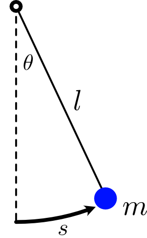
The $F = ma$ equation for its coordinate $\theta$, which measures the angle of the pendulum, looks like this:
$$ \frac{\mathrm{d}^2\theta}{\mathrm{d}t^2} = - \frac{g}{l} \sin \theta. $$
That’s due to the component of gravity $g \sin \theta$ that points along the direction of the pendulum’s swinging. For a review of that, see my lesson all about pendulums.
And yet, this differential equation in general doesn’t have a simple solution for $\theta(t)$! At least, not in terms of familiar functions like $\sin$’s, $\cos$’s, $\frac{1}{2}gt^2$’s, and so on.
The reason for the difficulty is the factor of $\sin\theta$ on the RHS, which makes this a non-linear differential equation. Our original harmonic oscillator equation was linear because it only involved single powers of $x$ and its derivatives. By contrast, if you were to expand out $\sin(\theta)$ in a Taylor series,
$$ \sin(\theta) = \theta - \frac{\theta^3}{3!} + \frac{\theta^5}{5!} - \cdots, $$
you can see that it involves infinitely many powers of $\theta$, and so this is a non-linear equation.
So we can’t just substitute in a simple cosine function here anymore and expect to get a solution. (Except in the special case when $\theta$ is small—again, see the lesson all about pendulums.) But we can still use energy conservation!
With a little geometry, you can write the total energy as
$$ E = \frac{1}{2} ml^2 \left(\frac{\mathrm{d}\theta}{\mathrm{d}t} \right)^2 -mgl\cos \theta. $$
The first term is the kinetic energy written in terms of $\theta$, and the second term is the gravitational potential energy $mgy$, where $y = -l \cos \theta$ is the height of the pendulum below the pivot point.
If we release the pendulum from rest at an angle $\theta(0) = \theta_0$, then the energy conservation equation says that
$$ \frac{1}{2} ml^2 \left(\frac{\mathrm{d}\theta}{\mathrm{d}t} \right)^2 -mgl\cos \theta = -mgl \cos \theta_0. $$
Once again, we can rearrange this equation to get the velocity $\frac{\mathrm{d}\theta}{\mathrm{d}t}$ as a function of $\theta$:
$$ \frac{\mathrm{d}\theta}{\mathrm{d}t} = \pm \sqrt{\frac{2g}{l}(\cos \theta - \cos \theta_0)}. $$
Now we separate the variables and integrate:
$$ \int \frac{\mathrm{d}\theta}{\sqrt{\cos\theta - \cos \theta_0}} = \pm \sqrt{\frac{2g}{l}} (t+c). $$
So far so good. At this point, however, the integral on the LHS is considerably harder than the one we saw before for the harmonic oscillator. It’s called an elliptic integral, and it doesn’t have a simple answer in terms of something like the $\cos^{-1}$ that we had before.
Fortunately, though, mathematicians a couple of centuries ago invested a huge amount of effort studying these kinds of integrals, and so a lot is known about their properties. The solution in this case can be written
$$ \theta(t) = 2\sin^{-1} \left( \sin\left(\frac{\theta_0}{2}\right)~ \mathrm{cd}\left(\Omega t \, \bigg|\, \sin^2\left(\frac{\theta_0}{2}\right)\right)\right), $$
where the devil is in that “$\mathrm{cd}$” function, called a Jacobi elliptic function.
The result looks like a simple cosine function when $\theta_0$ is small, but for large initial angles it changes dramatically.
So, this pendulum example shows how energy conservation can give us a different way to make progress with a challenging, non-linear differential equation, even when our first substitution method fails.
But now let’s get back to the harmonic oscillator equation,
$$ \frac{\mathrm{d}^2x }{\mathrm{d} t^2 } = -\Omega^2x. $$
So far, we’ve seen two ways of solving it. And these will more or less do the job for most of the equations you’ll meet in your first mechanics class. But if you’re up for it, what I’d like to do now is show you some more powerful methods that will come in handy later on when you’re faced with harder equations.
Method 3: Series Expansion
Using a series expansion is probably the most versatile of all the strategies I’ll show you in this lesson, and you can apply it to most any differential equation to get an exact, or even just an approximate solution.
The idea is, whatever the solution $x(t)$ to our differential equation might be, we can almost always expand it as a Taylor series in powers of $t$—at least within a window where things are well-behaved:
$$ x(t) = a_0 + a_1 t + a_2 t^2 + a_3 t^3 + a_4 t^4 + a_5t^5 + \cdots. $$
The question is, how do we figure out what these coefficients are supposed to be?
Let’s start off by imposing our initial conditions. When we plug $t = 0$ into the series expansion, all of the $t$’s disappear, and we’re left with $x(0) = a_0$. So we want to set $a_0=x_0$ to coincide with the initial position of the block.
And to impose that the initial velocity is zero, we’ll take the derivative of the series:
$$ \frac{\mathrm{d}x}{\mathrm{d}t} = a_1 + 2a_2 t + 3a_3t^2 + 4a_4 t^3 + 5 a_5 t^4 + \cdots. $$
Now when we plug in $t = 0$, we’re left with $a_1$, and so we want to set $a_1=0$.
Alright then, so far we’ve figured out $a_0$ and $a_1$. But there are still infinitely many coefficients left to determine!
The next thing we need to do is actually plug the expansion into the differential equation,
$$ \frac{\mathrm{d}^2x}{\mathrm{d}t^2} +\Omega^2 x = 0. $$
We’ll need to take the derivative of the series one more time to get the acceleration:
$$ \frac{\mathrm{d}^2x}{\mathrm{d}t^2} = 2a_2 + 3\cdot 2 a_3 t +4\cdot 3 a_4 t^2 + 5 \cdot 4a_5 t^3+\cdots. $$
And now we add on $\Omega^2 x$ and set the whole thing equal to zero. And we can pair up the corresponding terms:
$$ \begin{align} \frac{\mathrm{d}^2x}{\mathrm{d}t^2} +\Omega^2 x =& (2a_2 +\Omega^2 x_0)\\ &+ (3\cdot 2 a_3) t\\ &+(4\cdot 3 a_4 + \Omega^2 a_2) t^2 \\ &+ (5 \cdot 4a_5 +\Omega^2 a_3)t^3\\ &+\cdots\\ =&0. \end{align} $$
All this needs to vanish if we want our series to solve the differential equation. And the only way that can happen for every time $t$ is if all the coefficients are separately equal to zero. Then the idea is to go term by term through this sum, and demand that each factor in parentheses is zero.
That second term with a single power of $t$ looks the simplest, so let’s start there. Its coefficient is $3\cdot 2 a_3$. For that to vanish, we need to set $a_3 = 0$.
But notice that there’s also an $a_3$ in the $t^3$ term. And once we plug in $a_3 = 0$ there, all that’s left of that coefficient will be $5 \cdot 4 a_5$. And so for that to vanish, we’ll also have to set $a_5 = 0$.
We’ve therefore found that $a_1 = a_3 = a_5 = 0$. And the same thing is going to happen for all of the odd terms. So we conclude that all the odd coefficients are equal to zero.
That’s already pretty nice, because it means we get to throw out half the terms in our expansion,
$$ x(t) = x_0 + a_2 t^2 + a_4 t^4 + \cdots. $$
Now on to the even terms. The 0th one says that
$$ 2a_2 + \Omega^2 x_0 = 0, $$
and so we can solve for $a_2$:
$$ a_2 = -\frac{1}{2} \Omega^2 x_0. $$
Next, for the $t^2$ term, we have
$$ 4 \cdot 3 a_4+\Omega^2 a_2 = 0. $$
After plugging in our solution for $a_2$, we can again solve to get $a_4$:
$$ a_4 = +\frac{1}{4!} \Omega^4 x_0. $$
We can already see the pattern that’s forming. The first few terms of our series solution are
$$ x(t) = x_0 -\frac{1}{2}x_0\Omega^2t^2 +\frac{1}{4!}x_0\Omega^4 t^4+\cdots. $$
Does that look familiar? Let’s simplify it a bit by pulling out the common factor of $x_0$, and we can also put together the $\Omega$’s and the $t$’s like this:
$$ x(t) = x_0 \left( 1 - \frac{1}{2} (\Omega t)^2 + \frac{1}{4!} (\Omega t)^4 +\cdots \right). $$
How about now—does this thing look like the Taylor series for any function you know?
That’s right! The sum in parentheses is just the Taylor series for the cosine! And so, reassuringly, we’ve once again found that
$$ x(t) = x_0 \cos (\Omega t). $$
Series expansions like this are an extremely versatile method for solving all kinds of differential equations. You shouldn’t expect that they’ll always sum up to something simple and pretty like this one, though, unless you happen to be looking at a special differential equation with a simple solution. But even if you can’t sum up the infinite series into a familiar function, that doesn’t make it any less useful or valid as a solution to the equation—as long as you’re looking at a point where the series converges.
Method 4: Integral Transforms
Let’s keep it going with our next method: using an integral transform to solve a differential equation.
Now, there are lots of kinds of integral transforms out there—including the Fourier transform, which my last lesson was actually all about—but the one that’s most useful for solving the problem we’re looking at today is called the Laplace transform.
And here’s what it is. The Laplace transform is an instruction to take our position function $x(t)$, multiply it by $e^{-st}$ with some new variable called $s$, and then integrate that over $t$ from $0$ all the way to $t = \infty$:
$$ \hat x(s) = \int\limits_0^\infty \mathrm{d}t~ e^{-st} x(t). $$
What’s left is a function of $s$, that I’ll denote by $\hat x(s)$.
Okay… well that sounds like a funny thing to do, especially if you’ve never seen it before. But we’ll see in a moment that this transformation has a magical property when it comes to differential equations.
But the way you should think about it, is that we have two “spaces” here: $t$-space, where our original function $x(t)$ lives, and $s$-space, where its Laplace transform $\hat x(s)$ lives.
To give a couple of examples, if $x(t)$ were a constant, like $x(t) = 1$, then it’s just a horizontal line in $t$-space. And you can show pretty easily that its Laplace transform in $s$-space, obtained by doing the above integral, is $\hat x(s) = \frac{1}{s}$:

Or, for our block on a spring, we’ve found—and we’re about to find again—that $x(t) = x_0 \cos \Omega t$ oscillates in $t$-space. And in $s$-space, the result of the integral is a rational function, $\hat x(s) = \frac{x_0s}{s^2 + \Omega^2}$:

Alright, so we can do this integral to go from $t$-space to $s$-space. But why the heck would we want to do such a thing? How does it help us solve a differential equation like our harmonic oscillator,
$$ \frac{\mathrm{d}^2x }{\mathrm{d} t^2 } = -\Omega^2x. $$
The reason is that the Laplace transform acts in a beautifully simple way on derivatives. Look at what happens when we plug $\frac{\mathrm{d} x}{\mathrm{d} t }$ into the Laplace transform integral:
$$ \widehat{\frac{\mathrm{d} x }{\mathrm{d} t }}(s) = \int\limits_0^\infty \mathrm{d}t~ e^{-st} \frac{\mathrm{d}x }{\mathrm{d} t }. $$
We can simplify this by integrating by parts. In other words, we’ll use the product rule,
$$ \frac{\mathrm{d} }{\mathrm{d} t } (e^{-st}x) = e^{-st} \frac{\mathrm{d} x}{\mathrm{d} t } - se^{-st} x, $$
in order to rewrite the integrand as
$$ e^{-st} \frac{\mathrm{d} x}{\mathrm{d} t }= se^{-st} x+\frac{\mathrm{d} }{\mathrm{d} t } (e^{-st}x). $$
And now we do the integral over $t$:
$$ \widehat{\frac{\mathrm{d} x }{\mathrm{d} t }}(s) = \int\limits_0^\infty \mathrm{d}t~ \left( se^{-st} x+\frac{\mathrm{d} }{\mathrm{d} t } (e^{-st}x) \right). $$
The first term here is just $s$ times the Laplace transform of $x(t)$. After all, $s$ is a constant as far as the integral over $t$ is concerned, and so we can pull it outside the integral to get $s \hat x(s)$.
As for the second term, it’s the integral of a derivative, and so we can write down the result immediately:
$$ \int\limits_0^\infty \mathrm{d}t~ \frac{\mathrm{d} }{\mathrm{d} t } (e^{-st}x)= (e^{-st}x(t))\bigg|^{t=\infty}_0. $$
When we plug in $t = \infty$, $e^{-st}$ goes to zero. ($s$ has to be a positive number here for the Laplace transform integral to have a chance of making sense in the first place.) Then we’re simply left with $-x(0)$ from the other end of the integral.
And so, we’ve been able to simplify the Laplace transform of $\frac{\mathrm{d} x}{\mathrm{d}t }$ as
$$ \widehat{\frac{\mathrm{d} x }{\mathrm{d} t }} = s \hat x(s) - x(0). $$
This is the property that makes the Laplace transform so useful for solving differential equations. It says that taking a derivative in $t$-space is the same as simply multiplying by $s$ in $s$-space—up to a shift by $x(0)$.
And that means the Laplace transform can turn a differential equation for $x(t)$ into an algebraic equation for $\hat x(s)$, because all the derivatives disappear!
Let’s see how that works for our harmonic oscillator equation. We’ll take the Laplace transform of both sides:
$$ \widehat{\frac{\mathrm{d}^2x }{\mathrm{d} t^2 }} = -\Omega^2 \hat{x}(s). $$
Since $\Omega$ is a constant, the RHS is just $-\Omega^2$ times the Laplace transform of $x$.
On the LHS, we need to use our derivative rule twice in a row in order to simplify the Laplace transform of $\frac{\mathrm{d}^2x }{\mathrm{d}t^2 }$. If we plug that into our derivative rule, we get
$$ \widehat{\frac{\mathrm{d}^2 x }{\mathrm{d} t^2 }} = s \widehat{\frac{\mathrm{d}x }{\mathrm{d} t }} - \frac{\mathrm{d} x}{\mathrm{d} t }(0). $$
And now if we apply the rule a second time to simplify $\widehat {\frac{\mathrm{d}x }{\mathrm{d} t }}$ on the right, we get
$$ \widehat{\frac{\mathrm{d}^2x }{\mathrm{d} t^2 }} = s ^2 \hat x(s) - s x(0) - \frac{\mathrm{d} x}{\mathrm{d} t }(0). $$
When we plug in our initial conditions $x(0) = x_0$ and $\frac{\mathrm{d} x}{\mathrm{d} t }(0) = 0$, we find that the Laplace transform of our differential equation is
$$ s^2 \hat x(s) - s x_0 = -\Omega^2 \hat x(s). $$
As promised, there are no more derivatives! The Laplace transform took our differential equation for $x(t)$ and turned it into an algebraic equation for $\hat x(s)$!
And this equation is much easier to solve. Just move the $\hat x$’s over to the LHS,
$$ (s^2 + \Omega^2)\hat x(s) = sx_0, $$
and then divide out the factor out front to get
$$ \hat x(s) = \frac{sx_0}{s^2 + \Omega^2}. $$
And that’s the solution to our problem! In $s$-space, anyway.
To finish the job, we just need to transform back to $t$-space. There’s a general formula for doing that, but in practice it’s often faster to just pull up a table of Laplace transforms—there’s a nice one on Wikipedia—and find the one you’re looking for.
In fact, I already mentioned that this rational function is the Laplace transform of
$$ x(t) = x_0 \cos \Omega t. $$
And therefore that’s the solution to our original equation.
So that’s method number 4. Starting from a linear differential equation, take the Laplace transform to try to turn it into an algebraic equation, which you can solve for $\hat x(s)$. And finally, transform back to get your solution for $x(t)$.
Method 5: Hamiltonian Flow
Alright, we’re in the home stretch now! And I saved maybe the most fascinating of all for last: Hamilton’s equations and flows on phase space.
We started out with the $F= ma$ equation for a block on a spring:
$$ m \frac{\mathrm{d}^2x}{\mathrm{d}t^2} = -kx. $$
Notice that the LHS is the same as $\frac{\mathrm{d}}{\mathrm{d}t} \left( m \frac{\mathrm{d}x}{\mathrm{d}t}\right)$, since $m$ is a constant. In other words, it’s the derivative of the momentum, $p = m \frac{\mathrm{d}x }{\mathrm{d} t }$:
$$ \frac{\mathrm{d}p}{\mathrm{d}t} = - kx. $$
That’s just Newton’s second law: the force is the rate of change of the momentum.
But mathematically, what that enables us to do is replace the single, second-order differential equation that we started with, with a pair of first order equations:
$$ \begin{align} &\frac{\mathrm{d}x}{\mathrm{d}t} = \frac{p}{m}\\ &\frac{\mathrm{d}p}{\mathrm{d}t} = -kx \end{align} $$
These are called Hamilton’s equations. I haven’t done anything fancy—this pair of equations contains the exact same content as $F = ma$—all I’ve done is split it up into two pieces. The first equation is the definition of the momentum, and the second is $F = \frac{\mathrm{d}p }{\mathrm{d}t }$. And if you take another derivative of the first equation and plug in $\frac{\mathrm{d} p}{\mathrm{d} t }$ from the second, you’ll get back the same second order equation we’ve been studying all along,
$$ \frac{\mathrm{d}^2 x}{\mathrm{d} t^2 } = -\frac{k}{m}x. $$
But working with the first-order equations has a couple of big advantages. To see why it’s helpful, let’s draw a picture with $x$ on the horizontal axis and $p$ on the vertical axis:

This picture is called the phase space, and each point in this plane tells us where the block is and what its momentum—or equivalently its velocity—is at any given instant.
So, for example, when we pull the block out to its initial position and then release it from rest, that initial state corresponds to the point shown above on the horizontal axis, where $x = x_0$ and $p = 0$.
After we let it go, the block is going to begin to move, and so these $x$ and $p$ coordinates are going to change with time. The corresponding point in phase space therefore moves around with time, and it traces out a curve, called a flow.
And flow really is a good name for it, because I want you to picture this plane like the surface of a pool of water with some current flowing around it. Then we take something like a ping-pong ball and set it down at the point for our initial conditions. Once we let it go, the current will carry the ball off, moving it around the surface of the water. The flow is the path that the ball follows through the water.
But what determines the shape and strength of the current that’s telling the ball where to move? Our differential equations, of course! We can write the pair of them as a single, vector equation:
$$ \frac{\mathrm{d}}{\mathrm{d}t} \begin{pmatrix} x\\p \end{pmatrix} = \begin{pmatrix}p/m\\ -kx \end{pmatrix}. $$
Again, $x$ and $p$ are the coordinates of the ping-pong ball on the surface of the water, and their time derivative is telling us the ball’s velocity vector at each point on this surface. So, over at our initial point, $x$ was positive and $p$ was zero. Then the horizontal component of the velocity vector is zero, and the vertical component is negative. So the velocity of the imaginary ping-pong ball points straight down at that point, as shown in the figure.
Likewise, we can go to each point $(x,p)$ in this plane and draw the velocity vector $(p/m, -kx)$ at that location. Those arrows are what tell us the “current” that’s swirling around this plane, and what dictates how the ping-pong ball will move:

You can see that they’re swirling around the origin—that’s the equilibrium point. And I’m using the colors to indicate how strong the current is: it’s smallest for the yellow arrows near the middle, and gets bigger for the red arrows farther out.
By following those vectors starting from our initial conditions with $x = x_0$ and $p = 0$, we can see that the flow is an ellipse that wraps around again and again as the block oscillates back and forth. And since we know the energy is a constant, these curves are just the contours of constant energy in the $xp$-plane.
This is definitely a more abstract way of thinking about the solution to our differential equation. Remember, the physical system here is the block sliding back and forth on this one dimensional line. So obviously, there isn’t actually any pool of water or ping-pong ball. Those are just useful mathematical constructs for picturing what’s going on.
But what this picture buys us is that we can very quickly understand what the motion of our system is going to look like without solving any differential equations. All we need to do is draw the arrows at each point in phase space that we get from the RHS of Hamilton’s equations, either by hand or better yet on a computer.
That’s already extremely useful. But Hamilton’s equations also give us a direct way of explicitly writing down the solution for a linear equation like the harmonic oscillator, and that’s the last thing I want to show you.
To see that, let’s express the pair of Hamilton’s equations as a matrix equation:
$$ \frac{\mathrm{d}}{\mathrm{d}t} \begin{pmatrix} x\\p \end{pmatrix} = \begin{pmatrix} 0 & \frac{1}{m}\\ -k & 0 \end{pmatrix} \begin{pmatrix}x\\ p \end{pmatrix}. $$
This looks reminiscent of a simple differential equation of the form
$$ \frac{\mathrm{d}}{\mathrm{d}t} z(t) = \alpha z(t), $$
which says that when we take the derivative of a function $z(t)$, we’re supposed to get back $z$ again, times a number $\alpha$. The solution is simple:
$$ z(t) = e^{\alpha t}z(0), $$
as we can check:
$$ \frac{\mathrm{d} }{\mathrm{d} t } e^{\alpha t}z(0) = \alpha \underbrace{ e^{\alpha t}z(0)}_{z(t)}. $$
Our matrix equation for the block on a spring is of essentially the same form, just with vectors and matrices now instead of single numbers:
$$ \frac{\mathrm{d}}{\mathrm{d}t} \begin{pmatrix} x(t)\\p(t)\end{pmatrix} = M \begin{pmatrix} x(t)\\p(t)\end{pmatrix}. $$
It says that the derivative of the vector $\begin{pmatrix} x(t)\\p(t)\end{pmatrix}$ is equal to itself, multiplied by a constant matrix
$$ M =\begin{pmatrix} 0 & \frac{1}{m}\\ -k & 0 \end{pmatrix}. $$
And the solution is just the matrix analogue of our simple equation for $z$:
$$ \begin{pmatrix} x(t)\\p(t)\end{pmatrix} = e^{tM} \begin{pmatrix} x(0)\\p(0)\end{pmatrix}. $$
That way, when we take the $t$ derivative, it brings down a factor of $M$ from the exponent, and we get back $M$ times the same vector again.
The catch is that $M$, and therefore $e^{tM}$, are now matrices instead of single numbers. But what does it even mean to take the exponential of a matrix? The answer is provided by the Taylor series for $e$:
$$ e^{tM} = I + tM + \frac{1}{2!} (tM)^2 + \frac{1}{3!} (tM)^3 + \frac{1}{4!} (tM)^4 +\cdots, $$
where $I$ is the $2\times 2$ identity matrix.
That might look like a nasty thing to try to compute, and it certainly can be in general. But for our matrix $M$ in this problem the answer works out in a beautiful and simple way.
Let’s start off by seeing what $M^2$ gives us:
$$ M^2 =\begin{pmatrix} 0 & \frac{1}{m}\\ -k & 0 \end{pmatrix} \begin{pmatrix} 0 & \frac{1}{m}\\ -k & 0\end{pmatrix}= \begin{pmatrix} -k/m & 0\\ 0 & -k/m \end{pmatrix}. $$
That’s convenient! $M^2 = -\frac{k}{m} I$ is just the constant $-\Omega^2$ times the identity matrix. That makes calculating the higher powers of $M$ very simple. For example, for $M^3$ we get
$$ M^3 = M^2\cdot M = -\Omega^2M, $$
for $M^4$ we have
$$ M^4 = M^2 \cdot M^2 = \Omega^4 I, $$
and so on.
Then the Taylor series for $e^{tM}$ is
$$ e^{tM} = I + tM - \frac{1}{2!} t^2\Omega^2I - \frac{1}{3!} t^3\Omega^2M + \frac{1}{4!} t^4\Omega^4I + \cdots. $$
You can see that there are two kinds of terms: the odd powers of $t$ that multiply an $M$, and the even powers that multiply the identity matrix $I$. Let’s organize them together:
$$ \begin{align} e^{tM} = &\left(1 - \frac{1}{2!} (\Omega t)^2+ \frac{1}{4!} (\Omega t)^4+ \cdots \right) I\\ &+ \frac{1}{\Omega}\left( \Omega t - \frac{1}{3!} (\Omega t)^3 + \cdots \right)M. \end{align} $$
To make the second line look nicer, I’ve also multiplied and divided by $\Omega$, so that the $t$’s and $\Omega$’s show up with the same number of powers.
Now some beautifully simple sums are again staring us in the face. On the first line, the sum in parentheses is just $\cos(\Omega t)$, and on the second line the sum is $\sin(\Omega t)$. And so the matrix exponential simplifies to
$$ e^{tM} = \cos(\Omega t) I + \frac{1}{\Omega} \sin(\Omega t) M. $$
Or, writing out the matrix,
$$ e^{tM} = \begin{pmatrix} \cos(\Omega t) & \frac{1}{m\Omega}\sin(\Omega t)\\ -m\Omega \sin(\Omega t) & \cos(\Omega t) \end{pmatrix}. $$
Thus, to get the solution to Hamilton’s equations, we act this matrix on our initial condition vector,
$$ \begin{pmatrix} x(t)\\p(t)\end{pmatrix} =\begin{pmatrix} \cos(\Omega t) & \frac{1}{m\Omega}\sin(\Omega t)\\ -m\Omega \sin(\Omega t) & \cos(\Omega t) \end{pmatrix} \begin{pmatrix} x_0\\0\end{pmatrix}, $$
and we find
$$ \begin{pmatrix} x(t)\\p(t)\end{pmatrix}= \begin{pmatrix} x_0 \cos(\Omega t) \\ -m\Omega x_0 \sin(\Omega t)\end{pmatrix}. $$
Lo and behold, we obtain $x(t) = x_0 \cos(\Omega t)$ yet again! And of course the second line is the corresponding momentum, $m$ times the derivative of $x(t)$.
So I hope I’ve convinced you of how powerful Hamilton’s method is, of converting a second-order equation into a pair of first-order equations. Both for explicitly solving the equation with the matrix exponential, but also for visualizing the behavior of the solution as a flow on phase space.
Conclusion
We’ve now seen how to solve the harmonic oscillator equation with five different, increasingly sophisticated techniques!
Again, nobody’s saying you actually should use Laplace transforms or matrix exponentials to solve such a simple differential equation. But as you work your way up in physics, you’re quickly going to start running into more challenging differential equations where the methods you’ve gotten a glimpse of here become invaluable.
And it’s always a good idea to start learning advanced tools like these by first seeing how to apply them to a simple setup where you already know the solution, before you jump straight into trying to solve much more difficult problems where these tools do become essential.
Let me wrap up with a few last comments. First, this was hardly a complete list. There are many different strategies for solving differential equations that I didn’t cover here, and the best one to use depends on the equation you’re trying to solve. For example, one of the most ubiquitous in physics is the method of Green functions, which is also one of my favorites. But that really deserves a dedicated lesson.
Second, a really useful approach for solving hard differential equations is to try to tackle them in a special limit where they become simpler. I talked more about that in my lesson about Taylor series.
And third, remember that it’s not cheating to use a computer to help you solve a differential equation. Either by finding an exact solution, or a numerical approximation to the solution. There are lots of different tools for doing that, but one place to start is just to type your equation into wolframalpha.com.
See also:
If you encounter any errors on this page, please let me know at feedback@PhysicsWithElliot.com.