The Math & Physics of Taylor Series
Math is the language that we use to describe the laws of nature as physicists. And there’s no way around it: if you want to understand physics, you’re going to have to learn a lot of math. Whether that’s calculus for understanding $F = ma$, linear algebra for quantum mechanics, or differential geometry for general relativity. But there are certain mathematical results that you will meet time and again throughout your physics education. And if I had to pick one formula that’s the most important for understanding physics, it would be this one, Taylor’s formula:
$$ f(x+\varepsilon) = e^{\varepsilon \frac{\mathrm{d} }{\mathrm{d} x }}f(x). $$
It shows up in virtually everything we do in physics. And in this lesson I want to explain how it works, and give you a few examples of its importance in different corners of physics.
You’ve probably learned this theorem before if you’ve taken a calculus class, though you might not have written it in this nice and compact way. I’ll show you that it’s equivalent to the Taylor series:
$$ f(x) = f(x_0) + f'(x_0)(x-x_0) + \frac{1}{2} f''(x_0)(x-x_0)^2 + \cdots, $$
that lets us expand any smooth function $f(x)$ in powers of $x$.
In the first half of the lesson, I’m going to explain where this incredibly important formula comes from and what it means. And then in the second half I’ll tell you about three applications in physics where it shows up—though you’d be hard pressed to find a chapter of any physics textbook where it’s not applied.
First, we’ll look at how the Taylor series enables us to understand the complicated equations that we often need to solve in order to understand some physical system by studying a limit where the equations simplify.
Second, I’ll show you how Einstein’s $E = mc^2$, or actually his more general formula $E = \sqrt{m^2c^4+p^2c^2}$ for the energy of a relativistic particle of mass $m$ and momentum $p$ correctly reproduces the more familiar kinetic energy $\frac{1}{2}mv^2$ for particles that aren’t moving too close to the speed of light. And also how the same Taylor series leads to the fine-structure correction to the energy levels of the hydrogen atom.
And third, we’ll look at how Taylor’s formula leads directly to the definition of the momentum operator in quantum mechanics.
So let’s start with the math, and understand what this formula is all about. And after that we’ll see how it applies to these three physics examples.

Say we have some function, $f(x)$. Here’s a random example. It looks really complicated. But instead of trying to understand the whole complicated function at once, let’s zoom in and look at it in a smaller region where it’s a lot simpler. Take this red point, for example. I've chosen the origin so that this is the point $x = 0$, so the height of the function is $f(0)$ there.
Let’s imagine that we’re explorers living on the graph of this function. We start out at this point $(0, f(0))$, and we want to understand the shape of the whole function by venturing out in either direction from there. Before we start exploring, all we can say is that the height of the function is this number, $f(0)$, at our starting point. For all we know, the whole function might just be a constant, $y = f(0)$—in other words, a horizontal line.
But now we take a little step away from our starting point. We discover that the height of the function has changed, so it’s not actually a horizontal line. Instead, it now looks like a sloped line: the tangent line to the point where we started. The slope of that tangent line is the derivative of the function at $x = 0$. We write it either as
$$ f'(0) = \frac{\mathrm{d} f }{\mathrm{d} x }\bigg|_{x = 0}, $$
where the notation $\frac{\mathrm{d}f }{\mathrm{d} x }$ stands for the rise over run: the tiny change $\mathrm{d}f$ in the height of the function when we take a tiny step $\mathrm{d}x$ to the right.
So now that we’ve explored this little neighborhood of $x = 0$, as far as we know our function is a straight line going through $(0,f(0))$ with slope $f'(0).$ The equation of this line is
$$ f(x) \approx f(0) + f'(0) x. $$
This is indeed a good approximation to the actual function $f(x)$ as long as $x$ is tiny, so that we haven’t strayed too far away from $x = 0.$
But now we explore a little farther. We discover that the height of the function is deflected away from this sloped line. It’s actually starting to look more like a parabola! So we record on our map that a better approximation would be
$$ f(x) \approx f(0) + f'(0) x + A x^2, $$
for some number $A$.
And as we venture farther still out into the wilderness, we discover that the function isn’t actually a parabola, and we ought to add $x^3$ and $x^4$ and $x^5$ terms in order to maintain a good approximation to it.
This is the idea behind the Taylor series. We take our function and try to expand it in powers of $x$:
$$ f(x) = C_0+C_1x+C_2 x^2 +C_3x^3 + \cdots, $$
where the coefficients $C_0,C_1,C_2,C_3,$ and so on, are numbers that depend on the function $f$. All we need to do is figure out how to choose them so that the right-hand-side here coincides with our function.
We’ve already seen what the first couple of coefficients are. When we plug in $x = 0$, we get
$$ f(0) = C_0, $$
so that first number is just the value of the function at our starting point $x = 0.$ As for $C_1$, that term and everything else disappears when we plug in $x = 0.$ But let’s take the derivative of this whole equation:
$$ f'(x) = C_1 + 2C_2x + 3 C_3x^2 + \cdots, $$
remembering the rule that the derivative of $x^n$ is $n x^{n-1}.$ Now when we plug in $x = 0,$ the $C_1$ term survives!
$$ f'(0) = C_1. $$
So, like we already knew, we should set this first coefficient $C_1$ to be the derivative of $f$ at $x = 0.$
But now we’ve got the idea. If we take the derivative again, we get
$$ f''(x) = 2C_2 + 3 \cdot 2 C_3 x + \cdots, $$
and so when we plug in $x = 0$ we learn
$$ f''(0) = 2C_2. $$
Then we should choose $C_2 = \frac{1}{2} f''(0)$ to be half the second derivative of $f$ at $x = 0.$ And on and on it goes. The next term is
$$ f'''(0) = 3 \cdot 2 C_3, $$
and so we set $C_3 = \frac{1}{6} f'''(0).$
Hopefully you see the pattern. For the $n$’th term in the series,
$$ f(x) = \cdots + C_n x^n, $$
we need to take the derivative $n$ times, until this is the only term that’s around when we plug in $x = 0:$
$$ f^{(n)}(0) = n(n-1)(n-2)\cdots2\cdot 1 C_n, $$
where $f^{(n)}$ stands for the $n$’th derivative of $f$. So the $n$’th coefficient is
$$ C_n = \frac{1}{n!} f^{(n)}(0), $$
where $n! = n(n-1)(n-2)\cdots2\cdot 1.$
Now we’re in business! The farther away from $x = 0$ we get, the more terms we need to include in our series in order to get a good description of the function. But now that we have the general formula for the coefficients, we can include as many terms as we like:
$$ f(x) = f(0) +f'(0)x + \frac{1}{2} f''(0) x^2 + \frac{1}{3!} f'''(0) x^3 +\cdots+\frac{1}{N!} f^{(N)}(0) x^N. $$
And here’s the kicker: when we include all the terms by summing up the infinite series over all powers of $x$, we reproduce the exact function that we started with, as long as the function was sufficiently well-behaved. This is truly remarkable. It says that if we know all the derivatives of a function at a single point, we can reconstruct the rest of the function everywhere else.

Let’s do some examples. How about $f(x) = \sin x$? Let’s write down its Taylor series around $x = 0.$ All we need to know are the derivatives evaluated there. So let’s make a little table:
$$ \begin{array}{l|l|l|l} &f^{(n)}(x) & f^{(n)}(0) & \frac{1}{n!} f^{(n)}(0)x^n\\ \hline n=0 & f(x) = \sin (x) & f(0) = 0 &\frac{1}{0!} f(0) = 0 \phantom{ \int}\\ n=1 & f'(x) = \cos(x) & f'(0) = 1 & \frac{1}{1!} f'(0)x = x \phantom{\int}\\ n=2 & f''(x) = -\sin(x) & f''(0) = 0 & \frac{1}{2!} f''(0) x^2= 0 \phantom{\int}\\ n=3 & f'''(x) = -\cos(x) & f'''(0) = -1 & \frac{1}{3!} f'''(0)x^3 = -\frac{1}{3!} x^3\phantom{\int}\\ n=4 & f''''(x) = \sin(x) & f''''(0) = 0 & \frac{1}{4!} f''''(0) x^4= 0 \phantom{\int} \end{array} $$
$\sin(x)$ passes through the origin, so we start off with $f(0) = 0$. $0!$ is defined as 1 by the way, so our formula for the coefficients still makes sense there. Next up, we need the derivative of $\sin(x)$—that’s $\cos(x)$. Now when we plug in $x = 0$ we get $f'(0) = 1$, and so the first interesting term here is just $x$: a straight line through the origin with slope 1. That’s already a very good approximation to $\sin(x)$ when $x$ is a small number, and so we use the approximation $\sin(x) \approx x$ often in physics.
But once $x$ gets a little bigger, clearly the straight line isn’t going to cut it anymore. So let’s keep going. For the next term, we need the derivative of $\cos(x)$, which is $-\sin(x)$. But that vanishes again when $x = 0$, so the $x^2$ term disappears. That’s part of the reason the linear approximation was so good to begin with.
Now for $f'''(x),$ we need the derivative of $-\sin(x)$, and we get $-\cos(x)$. Then $f'''(0) = -1$, and so the cubic term is $-\frac{1}{3!} x^3.$ Then so far we’ve got
$$ \sin(x) \approx x -\frac{1}{3!} x^3. $$
Now we’ve got to do it again—but don’t worry, this will be the last derivative we have to take. For $f''''(x)$, we want the derivative of $-\cos(x)$, which is $\sin(x)$. In particular, $f''''(0) = 0$, and there’s no $x^4$ term.
Notice that this fourth derivative brings us back to where we started with $\sin(x)$. So this sequence of derivatives, $0,1,0,-1,$ is just going to repeat over and over again. And now we can just write down the whole series if we want without any more work:
$$ \sin(x) = x -\frac{1}{3!}x^3 +\frac{1}{5!}x^5 - \frac{1}{7!}x^7 + \frac{1}{9!}x^9 + \cdots. $$
When we add up the whole series, we get back the exact function, $\sin(x)$. Notice that only odd powers of $x$ show up on the right hand side. That’s because $\sin(x)$ is an odd function: when you compare it on the right and left sides of the $y$ axis, it looks the same except that it’s been flipped over. In other words, $\sin(-x) = - \sin(x).$ Then we can’t get any even powers in the Taylor series because they wouldn’t respect this property.
But oftentimes in physics we’re not interested in the whole series; what we really want is a good approximation to a function that makes a problem simpler to solve. I’ll show you examples of what I mean in a minute. In this case, we might stop with the first term and just apply the fact that $\sin(x) \approx x$ when $x$ is small. This is called the small-angle approximation, and you may have run into it when you learned about the simple pendulum.
The key point here is that when $x$ is small, like, say, $x = 0.1$, when we take larger powers of $x$ in the successive terms in the Taylor series, they get even smaller: $x^3 = 0.001,$ $x^5 = 0.00001$, and so on, not to mention the huge factorials in the denominators. That’s why we can ignore the higher order terms for small $x$, and get a good approximation to our function by keeping only the leading term.

Let’s do another quick example: $f(x) = e^x$. This one’s easy because the derivative of $e^x$ is just $e^x$ again. Then all the derivatives that we need to calculate the Taylor series are the same:
$$ f^{(n)}(x) = e^x \implies f^{(n)}(0) = 1. $$
So we don’t even need to make a table for this one, we can just jump right to the Taylor series:
$$ e^{x} = 1+x+\frac{1}{2}x^2+\frac{1}{3!} x^3 + \frac{1}{4!} x^4+\cdots. $$
This time none of the coefficients vanish. We get every power $x^n$, divided by $n!$. As a matter of fact, this infinite series is often take as the definition of $e^x$. And once again, if $x$ is tiny then we can get a good approximation by stopping at the linear term,
$$ e^x \approx 1+x. $$
We were able to reproduce the full functions $\sin(x)$ and $e^x$ by summing up their infinite Taylor series. But a word of warning: this isn't always possible. For example, another function that often shows up in physics is
$$ f(x) = \frac{1}{1-x}. $$
Try computing its Taylor series for practice: it's given by
$$f(x) = 1 + x + x^2 + x^3 + \cdots.$$
You might recognize this sum: it's the geometric series, and $f(x)$ is what you get when you add it all up. But notice that there are no $n!$ factors in the denominators here, like there were for, say, $e^x$. Then if $x$ is bigger than 1, the terms in this series just get larger and larger as the powers grow. That means the sum diverges for $x> 1.$
What went wrong? $f(x)$ is misbehaving! When $x = 1$, the denominator goes to zero, and the function blows up. Then the Taylor series breaks down beyond this point.
Now before we get to the physics examples, the last thing I want to do is show you a few convenient ways of writing Taylor’s formula. Spelling out the whole sum
$$ f(x) = f(0) + f'(0)x + \frac{1}{2} f''(0) x^2 + \frac{1}{3!} f'''(0) x^3+\cdots $$
isn’t very concise, but we can write the same thing much more compactly using summation notation:
$$ f(x) = \sum_{n=0}^\infty \frac{1}{n!}f^{(n)}(0) x^n. $$
This is the Taylor series for $f(x)$, expanded around $x = 0.$ But come to think of it, there was nothing special about $x = 0$ here; that’s just where we happened to put the origin when we drew the graph of $f(x).$ We could just as well write the expansion around any other point, call it $x_0$, like this:
$$ f(x) = \sum_{n=0}^\infty \frac{1}{n!}f^{(n)}(x_0) (x-x_0)^n. $$
Now we’re writing the series in powers of $x-x_0$—which measures how far away you are from the starting point $x_0$—and the coefficients are determined by the derivatives of $f$ at $x_0.$
Another convenient way to write the same thing is to define $\varepsilon = x - x_0$ as the distance away from $x_0.$ So when $\varepsilon$ is small you’re looking at the function near the starting point and as $\varepsilon$ gets bigger you get farther away. Then by plugging in $x = x_0+\varepsilon$ here, we could just as well write
$$ f(x_0+\varepsilon) = \sum_{n=0}^\infty \frac{1}{n!}f^{(n)}(x_0) \varepsilon^n. $$
This way of writing things makes it really clear that we can think of the Taylor series as starting out at the point $x_0$ and then expanding out away from there, by evaluating $f$ at $x_0+\varepsilon$ in powers of the displacement.
But that’s not even the slickest way to write the Taylor series, which is the formula I showed you at the very beginning. Remember our other notation for the derivatives,
$$ f^{(n)}(x) = \frac{\mathrm{d}^n f}{\mathrm{d} x^n }. $$
Moreover, we can think of $\frac{\mathrm{d}^n }{\mathrm{d} x^n }$ as an operator that takes a function, and then applies the derivative to it $n$ times:
$$ \frac{\mathrm{d}^n }{\mathrm{d} x^n } =\underbrace{ \frac{\mathrm{d} }{\mathrm{d} x } \frac{\mathrm{d} }{\mathrm{d} x }\cdots\frac{\mathrm{d} }{\mathrm{d} x }}_{n~\mathrm{times}} = \left( \frac{\mathrm{d} }{\mathrm{d} x }\right)^n. $$
Then we can also write the Taylor series as
$$ f(x+\varepsilon) = \sum_{n=0}^\infty \frac{1}{n!} \left( \frac{\mathrm{d} }{\mathrm{d} x }\right)^n f(x) \varepsilon^n. $$
I’ve dropped the $0$ subscript on $x$ now to keep things from getting cluttered, because that was just an arbitrary label. Dragging that $\varepsilon$ to the left inside the parentheses, we get
$$ f(x+\varepsilon) = \sum_{n=0}^\infty \frac{1}{n!} \left( \varepsilon\frac{\mathrm{d} }{\mathrm{d} x }\right)^n f(x). $$
Now this looks really interesting. It says that if we want to know the value of our function $f$ at a point that’s shifted away from $x$ by an amount $\varepsilon,$ what we should do is apply this special combination of derivatives to it:
$$ \sum_{n=0}^\infty \frac{1}{n!} \left( \varepsilon \frac{\mathrm{d} }{\mathrm{d} x }\right)^n. $$
But hang on a second—that looks familiar! Remember that the Taylor series we found for $e^z$ a minute ago was
$$ e^z = 1 + z + \frac{1}{2!}z^2 + \frac{1}{3!} z^3 + \cdots, $$
or, in sum notation,
$$ e^z = \sum_{n=0}^\infty \frac{1}{n!} z^n, $$
where I’ve written the variable with a new label $z$ so we don’t get it confused with $x.$ But that’s exactly what this differential operator looks like, with $z = \varepsilon \frac{\mathrm{d} }{\mathrm{d} x }$. Therefore, at least formally, we can express the full Taylor expansion in the form
$$ f(x+\varepsilon) = e^{\varepsilon \frac{\mathrm{d} }{\mathrm{d} x }} f(x). $$
This is the most compact, convenient, and beautiful way of writing Taylor’s formula. Just to make sure it’s clear how this works, let’s try applying it to a really simple function: $f(x) = mx+b.$ Obviously the Taylor series for this one is going to be really boring—it already is its own Taylor series! But let’s see what the formula says.
$$ e^{\varepsilon \frac{\mathrm{d} }{\mathrm{d} x }}(mx+b) = \left( 1 + \varepsilon \frac{\mathrm{d} }{\mathrm{d} x } + \frac{1}{2} \varepsilon^2 \frac{\mathrm{d}^2 }{\mathrm{d} x^2 } +\cdots\right)(mx + b). $$
First we expand out the derivatives by remembering the definition of the exponential as an infinite series. But most of the terms here aren’t going to contribute anything at all: our function is a straight line, and so everything from the second derivative on up will just give zero when it acts on $mx + b$.
So, from the “$1$” acting on $f$ we get $mx+b$. And from the $\varepsilon \frac{\mathrm{d} }{\mathrm{d} x }$, we get $\varepsilon m$. Then adding them up we find
$$ mx+b + m\varepsilon = m(x+\varepsilon)+b. $$
Which is precisely $f(x+\varepsilon)$, just as expected!
One last beautiful thing about this way of writing Taylor’s formula. It makes the generalization to the multi-variable Taylor expansion really straightforward. In other words, say we have a function $f(x,y,z) = f(\boldsymbol r)$ of three variables, where $\boldsymbol r = (x,y,z)$ is the position vector. For example, this might be the potential energy function of a particle moving around in three-dimensional space. Then what’s the Taylor expansion of this?
One way to approach it is to take $f(x+\varepsilon_x, y+\varepsilon_y,z+\varepsilon_z)$ and expand it, one variable at a time. For example, applying the Taylor expansion in $x$ we get
$$ f(x+\varepsilon_x,y+\varepsilon_y,z+\varepsilon_z) = f(x,y+\varepsilon_y,z+\varepsilon_z) +\varepsilon_x \frac{\partial }{\partial x }f(x,y+\varepsilon_y,z+\varepsilon_z) +\frac{1}{2}\varepsilon_x{}^2 \frac{\partial^2 }{\partial x^2 }f(x,y+\varepsilon_y,z+\varepsilon_z) + \cdots. $$
$\frac{\partial }{\partial x }$ here stands for the partial derivative with respect to $x$. All it means is that we should take the derivative of $f(x,y,z)$ with respect to $x$ like we normally would, treating the other variables $y$ and $z$ as constants.
But now we have to do the same expansion over again in each of these terms for $y,$ and then again in each of those terms for $z$. It’s a bit of a mess. But our exponential formula makes the whole thing incredibly simple. All we need to do to generalize
$$ f(x+\varepsilon) = e^{\varepsilon \frac{\mathrm{d} }{\mathrm{d} x }}f(x) $$
to multiple dimensions, is to replace $x \to \boldsymbol r = (x,y,z)$ with the position vector, $\varepsilon \to \boldsymbol \varepsilon = (\varepsilon_x,\varepsilon_y,\varepsilon_z)$ with the displacement vector, and $\varepsilon \frac{\mathrm{d} }{\mathrm{d} x }$ with the sum over all three directions:
$$\varepsilon_x \frac{\partial }{\partial x } + \varepsilon_y \frac{\partial }{\partial y } +\varepsilon_z \frac{\partial }{\partial z }.$$
We can write that more compactly as the dot product $\boldsymbol \varepsilon \cdot \nabla$ between $\boldsymbol\varepsilon$ and the “vector” of partial derivatives
$$ \nabla = \left( \frac{\partial }{\partial x }, \frac{\partial }{\partial y }, \frac{\partial }{\partial z }\right), $$
which is called “del.”. Then the multi-variable Taylor series is simply
$$ f(\boldsymbol r+ \boldsymbol \varepsilon) = e^{\boldsymbol \varepsilon \cdot \nabla} f(\boldsymbol r). $$
Okay, that’s enough math. Now let’s get to the physics. I promised to show you three applications:
- “Linearizing” complicated equations of motion
- The non-relativistic limit of $E = \sqrt{m^2 c^4 + p^2c^2}$ and the fine structure of hydrogen
- Defining the momentum operator in quantum mechanics
Let’s go one by one. You don’t necessarily need to know anything going in about relativity or quantum mechanics, by the way. The point is just to see how Taylor’s formula appears in several very different areas of physics.
Starting with number one. The basic procedure to solve a problem in classical mechanics is to write down all the forces on a particle, add them up and write $F = ma$, and then solve this equation for the position of the particle as a function of time.
That’s easier said than done, though. Especially the last step—solving $F = ma$—because for all but the simplest systems, this equation quickly becomes too hard to solve exactly. $F = ma$ is a differential equation, which just means that it contains derivatives of the function that you’re trying to solve for. And differential equations are much harder to solve than the algebraic equations that we all first learn in middle school and high school.
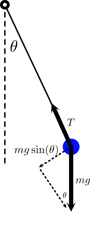
A simple example that I’ve told you about in a few past lessons is the pendulum. When solving for the motion of a pendulum, the main force we’re interested in is the component of gravity that points along the tangent direction to the circle where the particle is constrained to move. That’s $mg\sin \theta$, where $\theta$ is the angle that the pendulum makes with the vertical axis. Then the $F = ma$ equation for $\theta$ reads
$$ ml\frac{\mathrm{d}^2\theta }{\mathrm{d} t^2 } = -mg\sin\theta, $$
or
$$ \frac{\mathrm{d}^2\theta }{\mathrm{d} t^2 } = -\frac{g}{l}\sin\theta. $$
Simple as this physical setup looks, this equation is already very complicated because of that factor of $\sin(\theta)$ on the right-hand-side. It makes this what we call a non-linear differential equation, which can be very nasty to try to solve.
On the other hand, when $\theta$ is small, you can picture a pendulum gently rocking back and forth like a grandfather clock. And that motion certainly doesn’t seem very complicated. Is it possible then that we can simplify this equation when $\theta$ is relatively small?
The Taylor series lets us do just that. Like we worked out before, the Taylor series for $\sin$ is
$$ \sin \theta = \theta - \frac{1}{3!} \theta^3 + \frac{1}{5!} \theta^5+\cdots. $$
But if $\theta$ is a small number, then the successive terms get tinier and tinier because we’re raising the already tiny number $\theta$ to a positive power. Then for tiny $\theta$’s, we can apply our small-angle approximation from earlier by keeping only the linear term, and so our $F = ma$ equation becomes
$$ \frac{\mathrm{d}^2\theta }{\mathrm{d} t^2 } \approx - \frac{g}{l} \theta. $$
That’s vastly simpler! There’s no $\sin\theta$ factor here anymore making this equation complicated and non-linear. By applying the Taylor series, we’ve been able to linearize the differential equation, to turn it into a problem we can solve much more easily in the limit when the pendulum isn’t too far away from equilibrium.
This is just the equation of a simple harmonic oscillator now, like a mass on a spring, and the general solution is
$$ \theta(t) = A \cos\left( \sqrt{\frac{g}{l}} t \right) + B \sin\left( \sqrt{\frac{g}{l}}t\right). $$
So the pendulum indeed rocks gently back and forth from side-to-side.
If you’ve been watching my most recent videos and all this looks familiar, it’s no accident. I told you a few weeks ago about how the first thing we should do in any physics problem is expand the potential energy function around a stable equilibrium point in a Taylor series:
$$ U(x) = U(0) + U'(0) x + \frac{1}{2} U''(0)x^2+\cdots. $$
I chose my coordinates here so that the equilibrium point is at $x = 0.$
The first term, $U(0)$, is a constant, and doesn’t matter; you’re always allowed to change what you call the “ground level” of your potential energy function and shift this constant away. The second term, meanwhile, vanishes because we’ve chosen to expand around a minimum of the potential, where $U'(0) = 0$. So, typically, the first interesting term in the Taylor expansion of a potential around equilibrium is the quadratic term, which is just like the potential energy $U = \frac{1}{2}kx^2$ of a block on a spring. This is why systems oscillate back and forth around their equilibrium position.
As for the force, that’s related to the potential energy by
$$ F = -\frac{\mathrm{d} U}{\mathrm{d} x }, $$
and therefore the Taylor series for the force on a particle near equilibrium starts with
$$ F =-U''(0)x+\cdots, $$
just like the spring force $F = -kx.$ In particular, the force is linear! So the trick I taught you about the simple harmonic motion you’ll discover when you expand the potential energy around a stable equilibrium point is secretly the same thing as linearizing the $F = ma$ equation!
Next, let’s look at the Newtonian limit of Einstein’s theory of special relativity. In Newtonian mechanics, a free particle has energy
$$ E = \frac{1}{2} m v^2. $$
Alternatively, if we plug in the momentum $p = m v$, we can write the same thing as
$$ E = \frac{p^2}{2m}. $$
This is the energy of a non-relativistic free particle with momentum $p$. Non-relativistic means that the particle isn’t moving very fast compared to the speed of light. When particles due approach the speed of light, some weird and wild things happen, that were discovered by Einstein one hundred and some years ago when he wrote down his special theory of relativity.
In special relativity, the energy of a free particle of mass $m$ and momentum $p$ is given by
$$ E = \sqrt{m^2 c^4+p^2c^2}, $$
where $c$ is the speed of light.
You’ve run into this before even if you’ve never studied special relativity. If the particle is at rest, so that $p = 0$, we get
$$ E = \sqrt{m^2c^4} = m c^2, $$
which might be the most famous equation in physics.
But when the particle is moving, we need this more general formula including the momentum $p$. This formula holds even if the speed of the particle approaches the speed of light (though the definition of $p$ is modified from the Newtonian formula). But on the other hand, we know what the energy is supposed to be when $p$ is small, $\frac{p^2}{2m},$ so how do we see that Einstein’s formula correctly reproduces Newton’s formula for a slow moving particle?
The idea is of course to apply the Taylor expansion of Einstein’s energy when $p$ is small. Let’s first of all rewrite the formula a little bit to make it more convenient by pulling the $m^2 c^4$ outside the square root:
$$ E = mc^2 \sqrt{1 + \frac{p^2}{m^2c^2}}. $$
This makes it clear that what we want to do is compute the Taylor series for $f(x) = \sqrt{1+x}$, when $x = \frac{p^2}{m^2c^2}$ is small.
Actually, let’s go ahead and work out a slightly more general Taylor series for
$$ f(x) = (1+x)^q, $$
where $q$ is some power. Our case with the square root is then $q = 1/2.$ Let’s make a table again to work out the first few terms of the Taylor series:
$$ \begin{array}{l|l|l|l} &f^{(n)}(x) & f^{(n)}(0) & \frac{1}{n!} f^{(n)}(0)x^n\\ \hline n=0 & f(x) = (1+x)^q & f(0) = 1 &\frac{1}{0!} f(0) = 1\phantom{ \int}\\ n=1 & f'(x) = q(1+x)^{q-1} & f'(0) = q & \frac{1}{1!} f'(0)x = qx \phantom{\int}\\ n=2 & f''(x) = q(q-1)(1+x)^{q-2}& f''(0) = q(q-1) & \frac{1}{2!} f''(0) x^2= \frac{1}{2}q(q-1)x^2 \phantom{\int} \end{array} $$
The first term is always just what you get by plugging in $x= 0$; that’s just $f(0) = 1$. Then for the next term, we take the derivative, which brings down a factor of $q$, and when we evaluate that at $x=0$ we get the linear term, $q x.$ Then we take the second derivative, which brings down an additional factor of $q-1$, and so the quadratic term is $\frac{1}{2} q(q-1)x^2$.
Then we have
$$ f(x) = 1 +qx+\frac{1}{2}q(q-1)x^2 + \cdots. $$
The first pair of terms,
$$ (1+x)^q \approx 1 + q x, $$
is another very useful approximation that comes up a lot in physics.
Now back to the relativistic energy, we just plug in $q = \frac{1}{2}$ and $x = \frac{p^2}{m^2 c^2}$. To first order we get
$$ E = mc^2 \left( 1+\frac{1}{2} \frac{p^2}{m^2c^2} + \cdots \right). $$
Expanding it out, we’ve got
$$ E = mc^2 + \frac{p^2}{2m}+\cdots. $$
The first term is $E = mc^2$ again; that’s what we get by evaluating the energy of a particle at rest in relativity, called the relativistic rest energy of the particle. It doesn’t have an analogue in Newtonian mechanics, but on the other hand it’s just a constant. And you’re always free to add a constant to the total energy without changing anything, just like you get to pick what you want to call ground level when you’re defining a potential energy. Different choices just shift the total energy by a constant.
As for the second term, there we see how the Taylor series reproduces precisely the kinetic energy $\frac{p^2}{2m} = \frac{1}{2}mv^2$ that we expect in Newtonian mechanics. Actually, I’m being slightly sloppy here because the definition of the momentum $p$ gets modified in relativity, and we should Taylor expand that as well. But in the non-relativistic limit we of course get back the Newtonian momentum $p \approx mv$.
So that’s how Einstein’s formula connects to $E = mc^2$ and what we’re used to thinking of as kinetic energy. But what about the next term in the Taylor series? That one comes from
$$ \frac{1}{2} q(q-1)x^2 = -\frac{1}{8} \frac{p^4}{m^4c^4}, $$
so that the energy is
$$ E = mc^2 + \frac{p^2}{2m}-\frac{p^4}{8m^3c^2}+\cdots. $$
Newtonian mechanics is a good description of the world for particles that aren’t moving anywhere close to the speed of light. But, like any theory of physics, it’s only an approximation to nature. This next term in the Taylor series is the leading relativistic correction to the Newtonian energy. When $\frac{p}{mc} \approx \frac{v}{c}$ is tiny, meaning that the speed of the particle is much less than the speed of light, then this additional term gives a very small correction to Newton’s result, and we can ignore it without losing much accuracy. But as the speed gets larger, this correction becomes increasingly important.
One place we can see this correction in action is in the binding energy of a hydrogen atom. That’s the amount of energy you would need to kick the electron out of its “orbit” around the proton at the center of the hydrogen atom. In a lesson from a couple of months ago, I showed you how we can get 90% of the way to the answer for the binding energy just by applying dimensional analysis: in other words, by making a list of the parameters we have available to play with and their units, and seeing how we can combine them to get something with the units that we want. In this case, we saw that we can combine the electron mass $m$, its electric charge $e$, Coulomb’s constant $k$ (which sets the strength of the electric force), and Planck’s constant $\hbar$ (which sets the scale of quantum mechanics),
$$ m \sim \mathrm{kg},\quad e \sim \mathrm{C},\quad k \sim \mathrm{\frac{N\cdot m^2}{C^2}},\quad \hbar \sim \mathrm{kg \cdot \frac{m^2}{s}}, $$
to get units of energy like so:
$$ E \propto\frac{m(ke^2)^2}{\hbar^2}. $$
Just by thinking about the units like this gets us almost all the way to the answer. The actual formula for the binding energy comes with a factor of half, which we can’t get by only thinking about units, because “2” doesn’t have any units:
$$ E =\frac{m(ke^2)^2}{2\hbar^2} + \cdots. $$
This is Bohr’s formula for the binding energy of hydrogen, and it was one of the first great accomplishments of quantum mechanics. Its numerical value, about $13.6~\mathrm{eV}$, matches very closely to the experimental value of the binding energy.
And yet, Bohr’s formula is only an approximation: it neglects the small, but fascinating and experimentally observable, effects of special relativity. But where did we go wrong in our dimensional analysis argument? We wrote down the only possible way to combine $m,e,k,$ and $\hbar$ to make units of energy.
Well, it’s not that we went wrong, per se, it’s that in writing down the non-relativistic approximation to the binding energy, we omitted the speed of light $c$ from our list of parameters. So if we want to consider the effects of special relativity, we need to consider how $c$ can enter the formula for the energy.
But something remarkable happens when we add $c$ to the list of parameters: we can form a dimensionless combination by
$$ \alpha = \frac{ke^2}{\hbar c}. $$
This combination $\alpha$ is called the fine-structure constant. I’ll leave it for you to check that all the dimensions really do cancel out here when you plug in the units. If you put in the numbers you’ll find that $\alpha\approx 0.0073$, or a little more memorably,
$$ \alpha \approx \frac{1}{137}. $$
Since $\alpha$ is unitless, dimensional analysis doesn’t tell us anything about how it appears in the formula for the energy—no more than dimensional analysis could tell us about the factor of 2 in the denominator. Any function of $\alpha$ can multiply our expression for the energy without spoiling the units. This is how relativity allows small corrections to Bohr’s formula—which, remember, was itself already an excellent approximation to the experimental value of the Hydrogen binding energy. But we can get an even better theoretical prediction by considering the relativistic corrections.
With the leading relativistic correction $-\frac{p^4}{8m^3c^2}$ that we derived by applying the Taylor series to Einstein’s formula, we can determine the small modification that relativity makes to Bohr’s formula. The details require quantum mechanics, so I won’t go into that here, but the result is that
$$ E =E_\mathrm{Bohr}\left( 1 + \frac{5}{4}\alpha^2 +\cdots\right), $$
where $E_\mathrm{Bohr}$ is Bohr’s original formula for the binding energy that ignored relativity. That’s what the first term here reproduces. The second term gives a very small correction to it, because $\alpha$ is a tiny number. It’s therefore called a fine-structure correction.
There are in fact further corrections to this formula, both at order $\alpha^2$, as well as even smaller corrections at higher orders in $\alpha,$ due to various interesting effects.
Finally, while we’re on the subject of quantum mechanics, let’s finish by seeing how Taylor’s formula is related to the definition of momentum in quantum mechanics. In classical mechanics, the main question is to solve for the trajectory $x(t)$ of a particle as a function of time. In quantum mechanics, on the other hand, the goal is to find the wavefunction $\Psi(x)$ describing the particle, and how it evolves with time. Where the (square of the) wavefunction is bigger, the more likely you are to find the particle at that location when you make a measurement.
The things that we measure about the particle, like its position and momentum, are represented by operators that act on the wavefunction. We write $\hat{{} x}$ for the operator that measures the position and $\hat{{} p}$ for the operator that measures the momentum. The goal isn't to learn quantum mechanics right now, but I gave you a bit of a crash course in the lesson about symmetries in quantum mechanics, if you're interested in learning more.
Classically, I’ve told you about how momentum is the generator of spatial translations, meaning that momentum defines a classical operation that picks up a particle and shifts it over a bit:
$$ p:x\to x+\varepsilon. $$
Quantum mechanically, we therefore expect the momentum to be related to an operator, call it $\hat{{} U}(\varepsilon)$, that shifts the wavefunction over by $\varepsilon$:
$$ \hat{{} U}(\varepsilon) \Psi(x) = \Psi(x-\varepsilon). $$
Don’t sweat the minus sign. It’s there because of the distinction between shifting the operator $\hat{{} x} \to \hat{{} x} + \varepsilon$, which is like picking up your coordinate system and moving it to the left, and shifting the wavefunction $\Psi(x) \to \Psi(x-\varepsilon)$ to the right. But let’s not worry about it right now, and just take this as the definition of the translation operator in quantum mechanics.
Well that looks familiar! Physics aside, $\Psi(x)$ is just a function, and this formula tells us that we’re looking for an operator that shifts the position where $\Psi$ is evaluated over by $\varepsilon$. That’s just what Taylor’s formula does!
$$ e^{-\varepsilon \frac{\mathrm{d} }{\mathrm{d} x }} \Psi(x) = \Psi(x-\varepsilon). $$
Therefore, we identify the translation operator $\hat {{}U}(\varepsilon)$ with
$$ \hat{{} U}(\varepsilon) = e^{-\varepsilon\frac{\mathrm{d} }{\mathrm{d} x }}. $$
In quantum mechanics, we usually write operators like this as
$$ \hat{{} U}(\varepsilon) = e^{-\frac{i}{\hbar} \varepsilon \hat{{} Q}}, $$
where $\hat{{} Q}$ is called the generator of the transformation. The $\hbar$ is there so that $\hat{{} Q}$ comes out with the right units, and the $i$ is there so that $\hat{{} Q}$ is real in an appropriate sense (called Hermitian). It's analogous to writing a complex number as $e^{i\theta}.$
Then in the case of the momentum operator, Taylor’s formula can equivalently be written
$$ e^{-\frac{i}{\hbar}\varepsilon\left( \frac{\hbar}{i}\frac{\mathrm{d} }{\mathrm{d} x }\right)} \Psi(x) = \Psi(x-\varepsilon). $$
Thus, the generator of translations is
$$ \hat{{} Q} = \frac{\hbar}{i} \frac{\mathrm{d} }{\mathrm{d} x }, $$
and this is the definition of the momentum operator $\hat{{} Q} = \hat{{} p}$ in quantum mechanics.
This is just a small selection of physics applications where Taylor’s formula shows up. But again, you’d really be hard-pressed to find any chapter of any physics textbook where Taylor’s formula isn’t applied. Keep your eyes open, and you’ll see it everywhere!
See also:
If you encounter any errors on this page, please let me know at feedback@PhysicsWithElliot.com.