Electric Field Fundamentals

Introduction

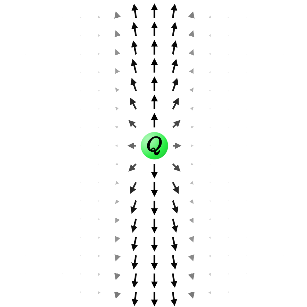
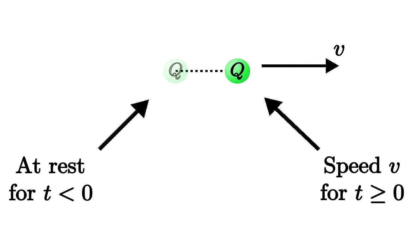
When you were first introduced to the idea of an electric field, you were probably shown something like the following picture of an electric charge $Q$ sitting at rest at the origin:

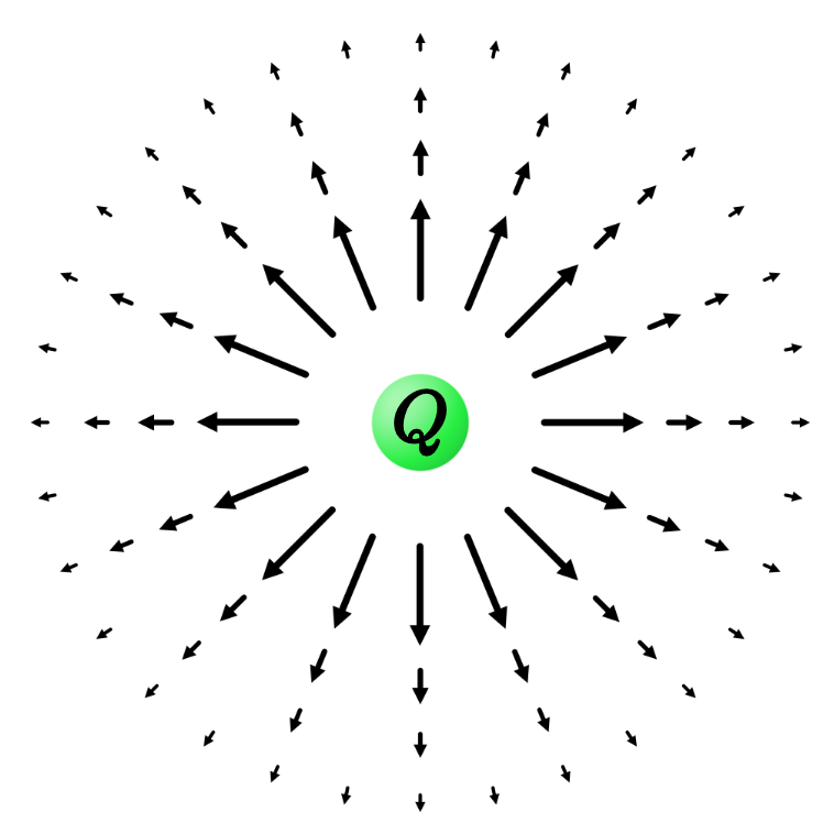
The electric field, you learned, is a collection of arrows—one for each point in space. The arrows point radially away from the charge, and they get shorter by a factor of $1/r^2$ the farther you get from the origin:

$$ E \propto \frac{Q}{r^2}. $$

That's all well and good when it comes to stationary charges. But it's important to understand that this simple picture is not the full story when it comes to the physics of electric (and, of course, magnetic) fields. The fields of moving charges can be quite different, especially as they approach the speed of light.

In particular, when charged particles accelerate, they launch electromagnetic waves out into the space surrounding them, like the ripples of a stone dropped into a pond. And in this lesson, we'll discover why.

Field Fundamentals

Let's start with a brief review of the fundamentals.

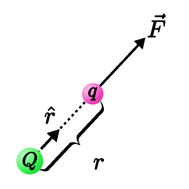
Picture a particle of charge $Q$ sitting at rest at the origin (the "source" charge). According to Coulomb's law, if any other charge $q$ is placed nearby (the "test" charge), it will experience an electric force along the line connecting the two charges,

$$ \vec F = k\frac{Qq}{r^2} \hat r, $$

where $\hat r$ is the unit vector pointing radially away from the origin.

The constant of proportionality $k$ is called Coulomb's constant, and it sets the strength of the electric force. For reasons that will become clearer later on, it's convenient to rewrite it in the slightly funny form

$$ k = \frac{1}{4\pi \epsilon_0}, $$

where $\epsilon_0$ is just another constant. Then the force that $Q$ exerts on $q$ is given by

$$ \vec F = \frac{1}{4\pi\epsilon_0} \frac{Qq}{r^2} \hat r. $$

If the two charges have the same sign, then their product $Qq$ is positive, and $\vec F \propto +\hat r$ points in the positive $r$ direction, meaning that $q$ is repelled away from $Q.$ If they have opposite signs, then $Qq$ is negative, $\vec F \propto -\hat r,$ and the test charge is attracted toward the source. To be concrete, let's suppose they're both positive.

At each point in space, we can draw the arrow that represents the force that the test charge $q$ would experience, were we to place it at that location. Or, better yet, we can draw the arrows that represent the force per unit test charge, $\vec F/q:$

$$ \frac{\vec F}{q} = \frac{1}{4\pi\epsilon_0} \frac{Q}{r^2} \hat r. $$

That way, the magnitude $q$ of the test charge disappears from the right-hand-side. The result is what we call the electric field, $\vec E$, produced by the source:

$$ \vec E(\vec r) = \frac{Q}{4\pi\epsilon_0} \frac{\hat r}{r^2}. $$

$\vec E(\vec r)$ is a vector field, meaning that it's a function that assigns an arrow to each point in space, as sketched in the picture at the top of the page. It tells us the electric force $\vec F(\vec r) = q \vec E(\vec r)$ that would be exerted on any test charge at that location by multiplying by $q$.

This simple formula—what I'll call the Coulomb field—describes the electric field sourced by a charge that's sitting at rest. It does not describe the electric field produced by a charge that's in motion—at least, not if it's moving anywhere close to the speed of light. One of the goals of this lesson is to determine the more general field of a moving charge.

Gauss's Law

Before we discuss moving charges, though, we need to talk about one of the fundamental equations of electromagnetism: Gauss's law.

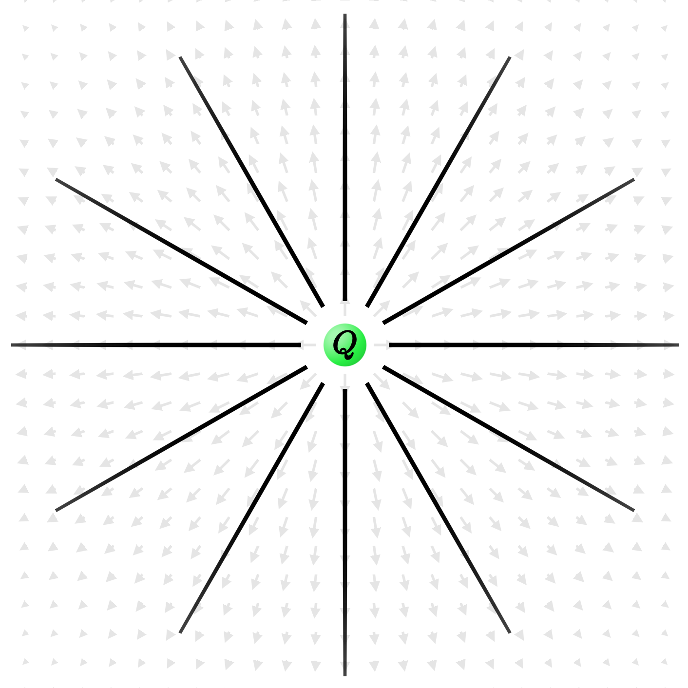
To motivate where it comes from, let's first discuss another useful way of visualizing the electric field. Rather than drawing the arrows at a smattering of sample points in space, we can connect them with streamlines that trace out the direction of the field at each point they pass through.

These are the particle's electric field lines, and they're reminiscent of the jets of water that you might see spraying out from a sprinkler. In fact, pushing that analogy a little further, if we wanted to measure the strength of a sprinkler, we could imagine surrounding the whole thing in a giant rubber balloon and measuring how much water per unit time is hitting its surface.

In a similar way, if we picture an imaginary sphere surrounding our point charge, then the strength of the field lines passing through the surface should give us a measure of the amount of charge contained inside.

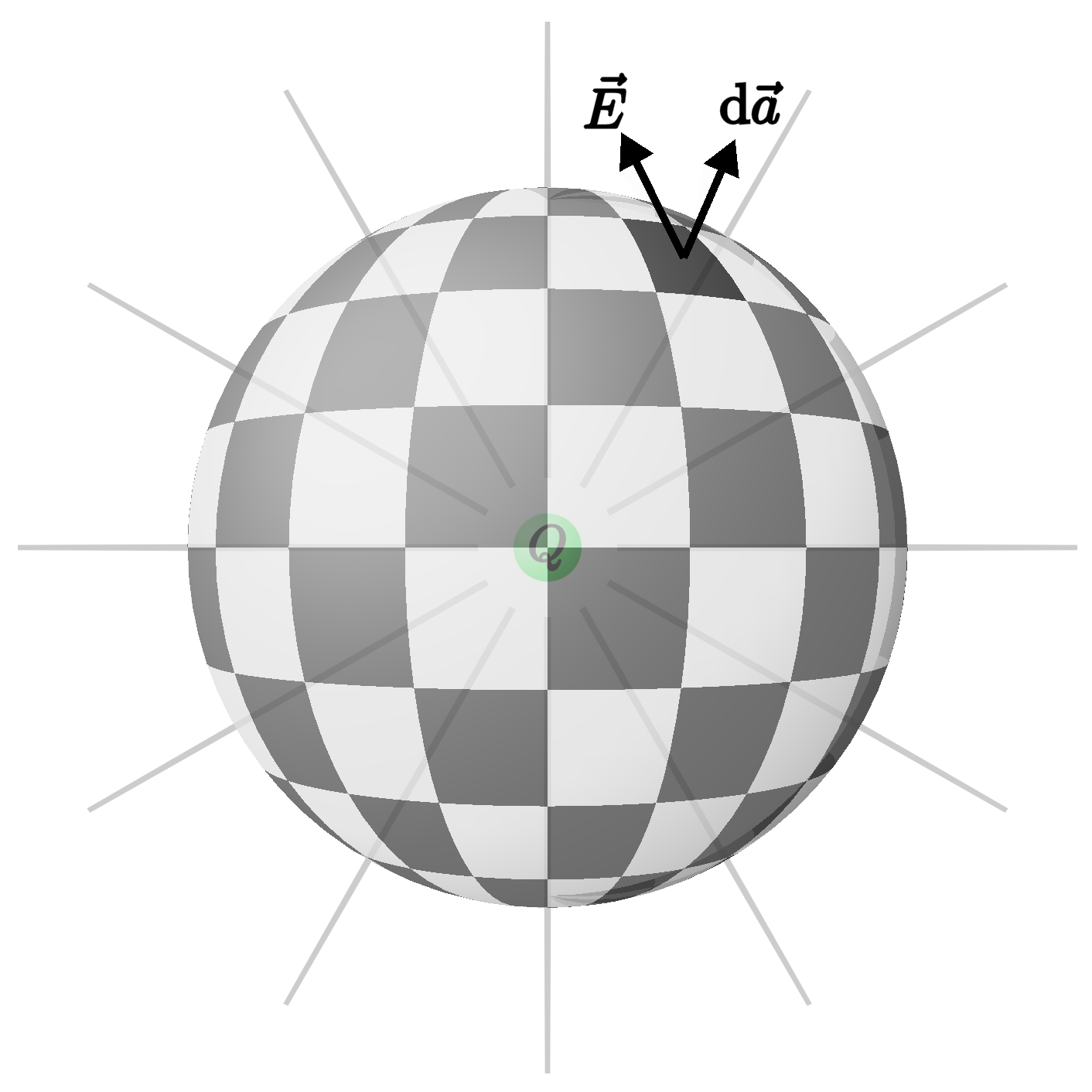
To make that idea precise, imagine slicing the surface up into lots of tiny patches. For each patch, we can construct a vector $\mathrm d \vec a = \hat n \,\mathrm da$, whose magnitude $\mathrm da$ is the area of the patch and whose direction $\hat n$ points perpendicularly away from the surface. In the case of a sphere, that normal direction coincides with $\hat r$, and we can write $\mathrm d \vec a = \hat r \, \mathrm da.$

By taking the dot product between that area vector and the electric field vector at the location of the patch, we get a number that quantifies the strength of the electric field that's passing outward through that tiny area—where the dot product serves to pick out the component of $\vec E$ that points through the surface as opposed to running parallel to it.

And, adding up the contributions from all the little patches making up the sphere by integrating over the entire surface,

$$ \Phi = \int_\mathrm S \vec E \cdot \mathrm d\vec a, $$

we obtain the electric flux, which measures the strength of the electric field passing outward through $\mathrm S$. In the sprinkler analogy, the flux would correspond to the amount of water flowing out per unit time through the balloon.

The analogy with the sprinkler suggests that the electric flux should be proportional to the amount of charge contained within the surface. So let's see what we get when we plug in our formula for the Coulomb field:

$$ \Phi = \int_{\mathrm S} \left( \frac{Q}{4\pi \epsilon_0} \frac{\hat r}{r^2} \right) \cdot \mathrm d \vec a. $$

Because we have spherical symmetry, the integral isn't hard to evaluate. Pulling the constant factors out front, including the constant radius $r=R$ of the sphere, we get

$$ \Phi = \frac{Q}{4\pi R^2\epsilon_0} \int_{\mathrm S}\hat r \cdot \mathrm d \vec a. $$

Substituting $\mathrm d \vec a = \hat r \, \mathrm d a$ for the area vector gives

$$ \Phi = \frac{Q}{4\pi R^2\epsilon_0} \int_{\mathrm S} \mathrm d a. $$

What remains of the integral is then just the area $\mathrm d a$ of each little patch, summed up over all the little patches making up the entire surface. In other words, it's the total area of the sphere, $4\pi R^2$.

The factors of $4\pi R^2$ then cancel—that's why it was convenient before to pull a factor of $4\pi$ out of Coulomb's constant, $k = 1/4\pi\epsilon_0.$ And so, as we'd hoped, the total electric flux passing through the surface has indeed told us the amount of charge $Q$ contained inside of it:

$$ \boxed{\int_\mathrm S \vec E \cdot \mathrm d \vec a = \frac{Q}{\epsilon_0}.} $$

This is Gauss's law; it's one of the central equations of electromagnetism. It holds for any configuration of electric charges, and for any surface $\mathrm S$ surrounding them—it doesn't necessarily have to be a sphere.

And it also holds not just for stationary charges like we've been considering so far, but also for charges that are moving with non-zero velocity. And that's the topic we'll turn to next.

The Field of a Moving Charge

As already emphasized, Coulomb's law describes the electric field of a stationary charged particle. The field of a rapidly moving charge can look quite different.

To keep things simple to begin with, let's consider a charge that's spent its whole life moving with constant speed $v$ to the right—we'll deal with accelerating charges later on. Then what does the electric field produced by this particle look like?

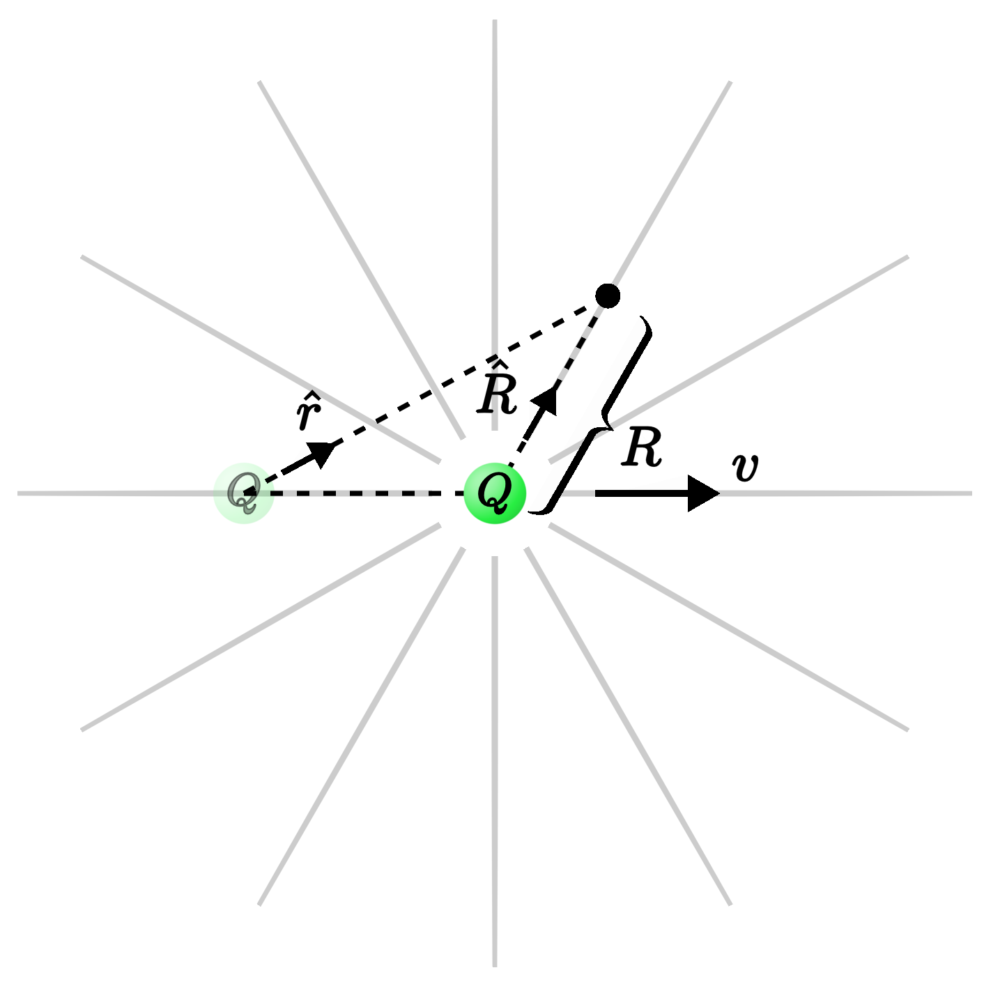
Your first guess might be that it looks about the same, except that the moving charge drags the usual Coulomb field along with it as it goes. In other words, instead of pointing in the radial direction away from the origin along $\hat r$, we'd guess that the field points radially away from the current position of the charge at time $t$.

If we call that new vector $\hat R$ and that new distance $R$, then the natural guess would be that the electric field of the moving charge is the same as our old Coulomb formula, but with all the little $r$'s replaced by big $R$'s that refer to the current position of the charge:

$$ \vec E \approx \frac{Q}{4\pi\epsilon_0} \frac{\hat R}{R^2}. $$

In fact, that's a very good approximation to the field—provided that the charge isn't moving too fast. But as the speed of the particle increases toward the speed of light, the shape of its electric field changes dramatically.

The field gets "squished" along the direction of motion, becoming very weak in the forward and backward directions, and conversely very strong in the perpendicular directions. And the easiest way to see why is to demand that the field is consistent with the principles of special relativity.

Thus, consider again the ordinary Coulomb field for a charged particle sitting at rest. If we hop on a train that's moving to the left at speed $v$ and look out the window, from the perspective of the train's frame of reference it's the particle that's now moving to the right at speed $v$. And therefore, by transforming the original Coulomb field from the particle's rest frame to the frame of the train, we can determine the electric field produced by the moving charge.

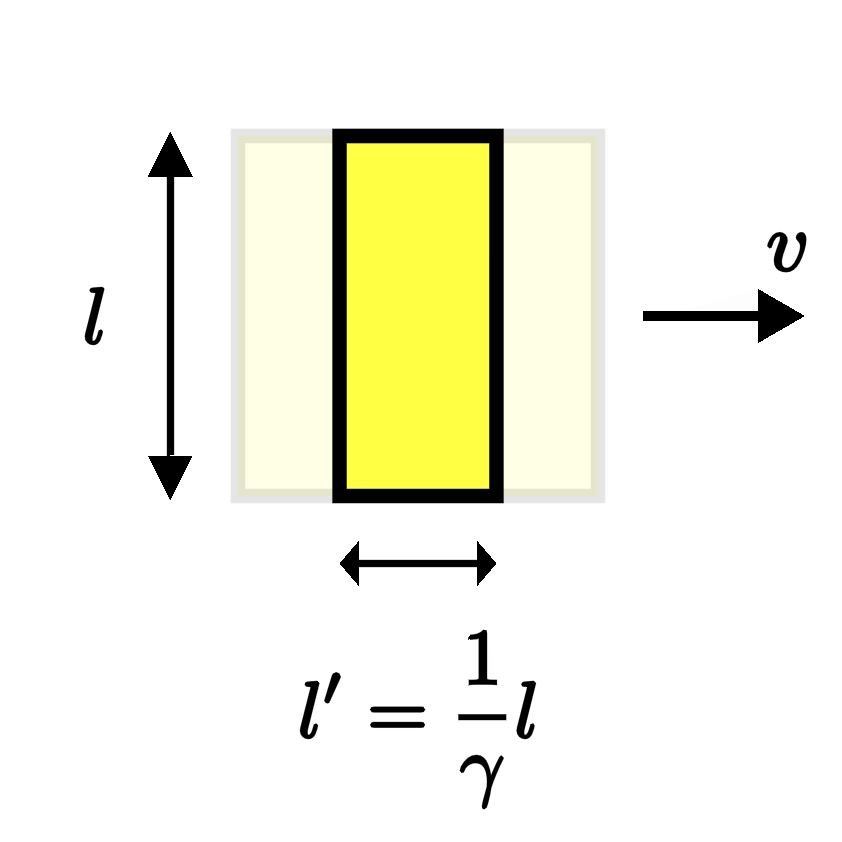
If you've studied a little special relativity before, the result is very similar to the effect of length contraction. For example, given a box of side length $l$ sitting at rest, if we set it moving to the right with speed $v$, then we'll find that its length is shortened along the direction of motion,

$$ l' = \frac{1}{\gamma} l, $$

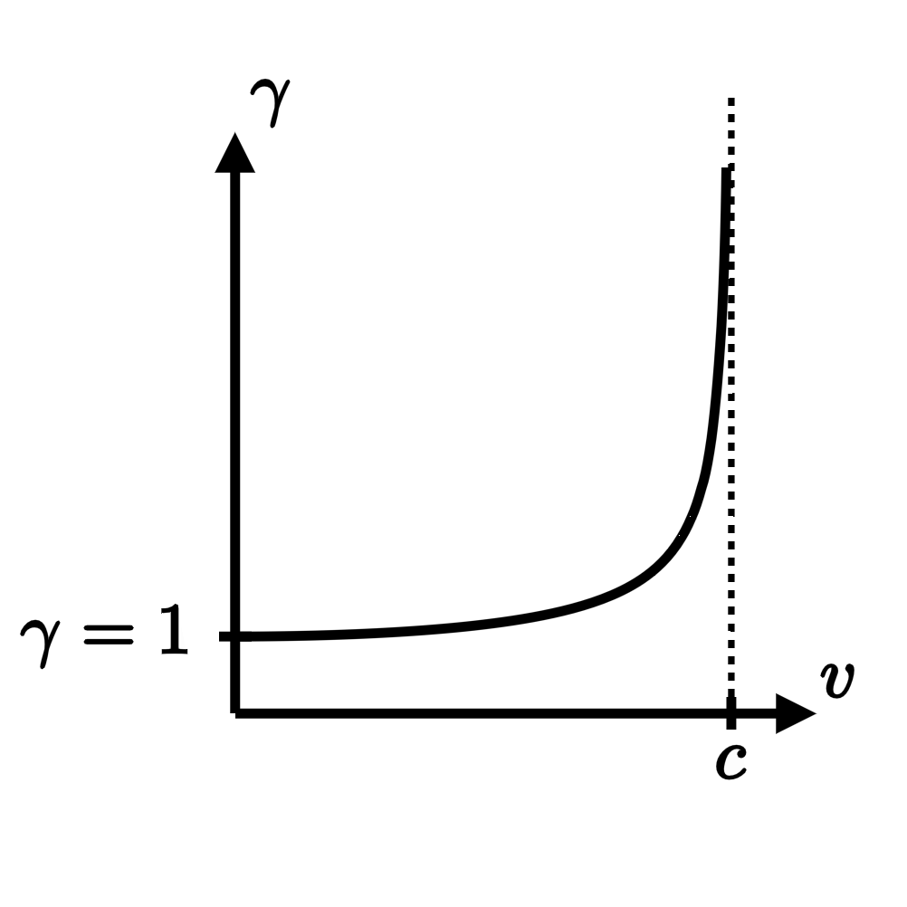
where the compression factor $\gamma$ is given by

$$ \gamma(v) = \frac{1}{\sqrt{1 - v^2/c^2}}. $$

When the speed $v$ is equal to zero, $\gamma=1$, and $l' = l$ reproduces the rest length of the box. But as $v$ increases and gets closer to the speed of light $c,$ $\gamma$ begins to blow up because its denominator approaches zero.

As a result, the box gets squished flatter and flatter along its direction of motion the faster and faster that it moves. And essentially the same effect leads to the squishing of the electric field of a moving particle when its speed is close to the speed of light.

As already discussed, the field is well-approximated by Coulomb's formula provided that $v$ is small. It points radially away from the charge along $\hat R$, and it has the same magnitude, proportional to $1/R^2$, in all directions surrounding the particle.

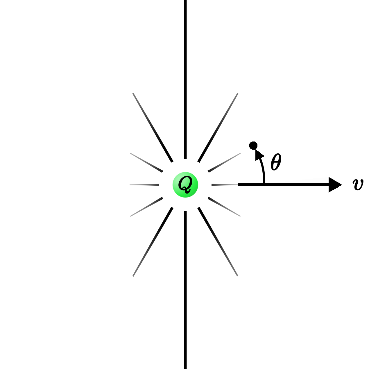
But as the speed increases, that spherical symmetry breaks, and the Coulomb approximation falls apart. Instead, the magnitude of the field is modified by an additional factor that depends on the angle $\theta$ between $\hat R$ and $\vec v:$

$$ \vec E = \frac{Q}{4\pi \epsilon_0} \frac{\hat R}{R^2}\left[\frac{1-v^2/c^2}{(1 - \sin^2(\theta) \,v^2/c^2)^{3/2}}\right]. $$

This is the generalization of Coulomb's law for a particle moving with constant velocity $\vec v$. We'll see how to derive it using the laws of special relativity in just a moment, but first let's investigate whether it reproduces the qualitative features that we would expect.

First, when $v$ is small compared to the speed of light, the factors of $v^2/c^2$ are close to zero, and the function in brackets approaches 1. In that case, we indeed get back the approximate Coulomb field of a slow-moving particle:

$$ \vec E \overset{v \ll c}{\longrightarrow} \frac{Q}{4\pi\epsilon_0} \frac{\hat R}{R^2}. $$

Spherical symmetry is restored in this limit because the factors of $\theta$ have disappeared.

If the particle is moving faster, however, we can no longer ignore those relativistic corrections. To understand their effect, let's examine the field directly in front of the particle, where $\theta = 0$:

$$ \vec E(\theta = 0) = \frac{Q}{4\pi \epsilon_0} \frac{\hat R}{R^2}\left[1-v^2/c^2\right]. $$

Compared to the usual Coulomb field, the value has been modified by a factor of $1/\gamma^2$:

$$ \vec E(\theta = 0) = \frac{1}{\gamma^2}E_\mathrm{Coulomb}. $$

Recalling that $\gamma$ becomes a large number as the particle nears the speed of light, we find that the electric field has been reduced by a large factor compared to Coulomb's formula directly in front of—and also behind—the moving particle.

In the perpendicular direction, on the other hand, where $\theta = \pi/2,$ we instead get

$$ \vec E(\theta = \pi/2) = \gamma \,E_\mathrm{Coulomb}, $$

meaning that the field has been amplified by $\gamma$ at right angles to the motion.

Thus, the field is indeed consistent with what we might have expected for the squashing of the field lines along the direction of motion, as motivated above. In fact, we can draw a picture of the magnitude of the field by making a polar plot of the function

$$ |\vec E(\theta)| \propto \frac{1-v^2/c^2}{(1 - \sin^2(\theta) \,v^2/c^2)^{3/2}} $$

with respect to the angle $\theta:$

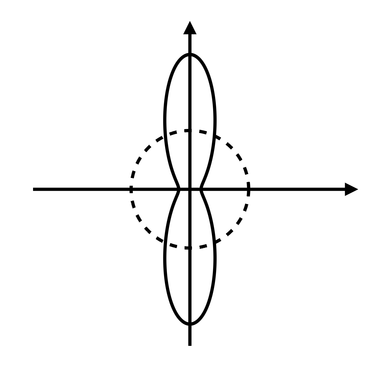
Here, the distance from the origin represents the magnitude of the field $|\vec E(\theta)|$ at the given angle. When the particle is sitting at rest (or moving slowly), the $\theta$ dependence disappears, and the polar plot simply traces out a circle. Thus, the magnitude of the electric field is the same in all directions surrounding the particle, as we would expect from Coulomb's law.

At higher speeds, however, the shape of the circle is deformed into something more like a peanut, showing again that the magnitude of the field is reduced in the directions in front of and behind the particle, and simultaneously increased at right angles to the motion.

Now that we've understood its qualitative features, let's return to the explicit derivation of the field of the moving charge. As explained above, we can determine it by applying the rules of special relativity.

Thus, let $F_0$ be the rest frame of the charge, with Cartesian coordinates $(x_0,y_0, z_0)$ and time coordinate $t_0.$ In this frame, the field is given by the usual Coulomb formula, which we can expand in Cartesian coordinates as

$$ \vec E_0 = \frac{Q}{4\pi\epsilon_0} \frac{x_0\hat x_0 + y_0\hat y_0 + z_0\hat z_0}{(x_0^2+y_0^2+z_0^2)^{3/2}}. $$

In other words, the electric field in this frame has components

$$ (E_{x_0}, E_{y_0}, E_{z_0}) = \frac{Q}{4\pi\epsilon_0} \frac{(x_0, y_0, z_0)}{r_0^3}, $$

where $r_0 = \sqrt{x_0^2+y_0^2+z_0^2}.$

Now let's transform to the "train frame" as described above. That is, consider another frame $F$ moving along the $-x_0$ direction with constant speed $v,$ with Cartesian coordinates $(x,y,z)$ and time coordinate $t$. From the perspective of this frame, the particle is moving along the positive $x$ direction with speed $v:$

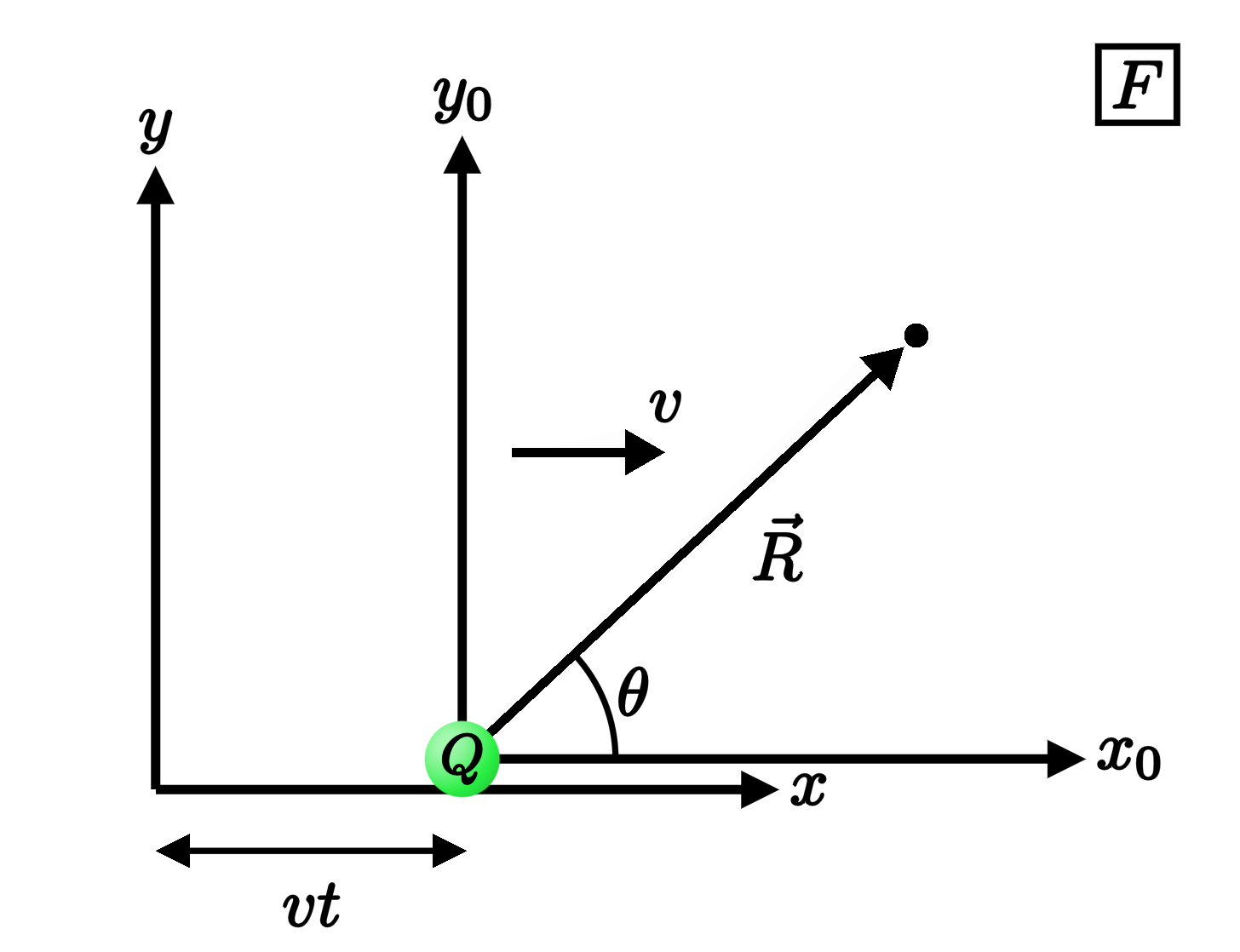
The coordinate systems for the two frames are related by a Lorentz transformation:

$$ \begin{aligned} &x_0 = \gamma(x - vt)\\ &y_0 = y\\ &z_0 = z\\ &t_0 = \gamma ( t - vx/c^2 ). \end{aligned} $$

The components of the electric field, meanwhile, transform according to

$$ \begin{aligned} &E_x = E_{x_0}\\ &E_y = \gamma E_{y_0}\\ & E_z = \gamma E_{z_0}. \end{aligned} $$

(If you're wondering where these formulas come from, see, for example, Ch. 5 of Purcell and Morin's Electricity and Magnetism or Ch. 12 of Griffiths's Introduction to Electrodynamics.)

The components of the electric field as measured in the frame where the charge is moving are therefore given by inserting factors of $\gamma$ in the $y$ and $z$ directions:

$$ (E_x, E_y, E_z) = \frac{Q}{4\pi\epsilon_0} \frac{(x_0, \gamma y_0, \gamma z_0)}{r_0^3}. $$

Plugging in the Lorentz transformations to replace $x_0,$ $y_0,$ and $z_0$ in the numerator, we get

$$ (E_x, E_y, E_z) = \frac{Q}{4\pi\epsilon_0} \frac{\gamma \,(x - vt, y, z)}{r_0^3}. $$

Note that the factor $(x-vt, y,z)$ that emerges corresponds to the components of the vector $\vec R = \vec r - vt \hat x$ pointing from the charge to the point where we're evaluating the field. Thus, we've so far shown that the electric field of the moving charge is given by

$$ \vec E = \frac{Q}{4\pi\epsilon_0} \frac{\gamma}{r_0^3} \vec R. $$

To complete the derivation, we need the following identity for $r_0:$

$$ r_0 = \gamma R \sqrt{1 - \sin^2(\theta)\, v^2/c^2}, $$

where $\theta$ is, as before, the angle between $\vec R$ and the axis of motion. To prove it, we'll plug the Lorentz transformation into $r_0 = \sqrt{x_0^2+y_0^2+z_0^2}:$

$$ r_0 = \sqrt{\gamma^2(x-vt)^2+y^2+z^2}. $$

From the geometry of the above figure, note that

$$ \cos \theta = \frac{x-vt}{R} \qquad \text{and} \qquad \sin \theta = \frac{\sqrt{y^2+z^2}}{R}. $$

We can therefore write

$$ r_0 = \sqrt{\gamma^2 R^2 \cos^2\theta + R^2 \sin^2 \theta}. $$

Replacing $\cos^2\theta = 1 - \sin^2 \theta,$ we get

$$ r_0 = R\sqrt{\gamma^2 + (1 -\gamma^2)\sin^2 \theta}. $$

Finally, making use of the identity $1 - \gamma^2 = -\frac{v^2}{c^2} \gamma^2$ that follows from the definition of $\gamma$, we arrive at the claimed identity for $r_0.$ Plugging it into our previous formula for the electric field, we obtain

$$ \vec E = \frac{Q}{4\pi\epsilon_0} \frac{\gamma}{\gamma^3 R^3(1 - \sin^2(\theta)\, v^2/c^2)^{3/2}} \vec R, $$

and, simplifying, we get $$ \vec E = \frac{Q}{4\pi\epsilon_0} \frac{1}{\gamma^2(1 - \sin^2(\theta)\, v^2/c^2)^{3/2}} \frac{\vec R}{R^3}. $$

Therefore, the electric field of a charge moving with velocity $\vec v$ is given by

$$ \vec E = \frac{Q}{4\pi\epsilon_0} \frac{1 - v^2/c^2}{(1 - \sin^2(\theta)\, v^2/c^2)^{3/2}} \frac{\hat R}{R^2}, $$

as claimed.

As we saw above, the appearance of the angle $\theta$ means that the spherical symmetry of the original Coulomb field has been broken. But we should expect as much, because we've singled out a special direction in space: the direction of motion of the charge.

Spherical symmetry or no, however, Gauss's law nevertheless applies. Meaning that if we once again surround the particle by an imaginary sphere—or any surface—and compute the total flux of the electric field passing through it, the result is still given by the charge $Q$ contained inside, divided by $\epsilon_0$. It's just that most of that flux now comes from the perpendicular directions where the field is strongest, rather than being uniformly distributed like it was for a stationary charge.

We can verify as much by once again computing the electric flux through a sphere of radius $R$ surrounding the particle,

$$ \Phi = \int \vec E \cdot \mathrm d \vec a. $$

Using spherical coordinates $\theta$ and $\phi$, the area element is given by $\mathrm da = R^2 \sin(\theta) \,\mathrm d \theta \,\mathrm d\phi.$ We therefore get

$$ \Phi = \frac{Q}{4\pi\epsilon_0} \int \frac{1 - v^2/c^2}{(1 - \sin^2(\theta)\, v^2/c^2)^{3/2}} \frac{\hat R}{R^2} \cdot \hat R~ R^2 \sin(\theta)\, \mathrm d \theta \, \mathrm d \phi. $$

There are no factors of $\phi$ in the integrand, so that integral simply contributes $\int_0^{2\pi} \mathrm d\phi = 2\pi$, leaving us with

$$ \Phi = \frac{Q}{2\epsilon_0} (1-v^2/c^2) \underbrace{\int_0^\pi \mathrm d \theta \, \frac{\sin (\theta)}{(1 - \sin^2(\theta)\, v^2/c^2)^{3/2}} }_{\frac{2}{1-v^2/c^2}}. $$

Evaluating the integral over $\theta$, the factors of $1-v^2/c^2$ cancel, and we're left with

$$ \Phi = \frac{Q}{\epsilon_0}, $$

as expected from Gauss's law.

Finally, before we move on to discuss the electric field of an accelerating charge, it's important to understand that a moving charge produces not just an electric field, but a magnetic field as well.

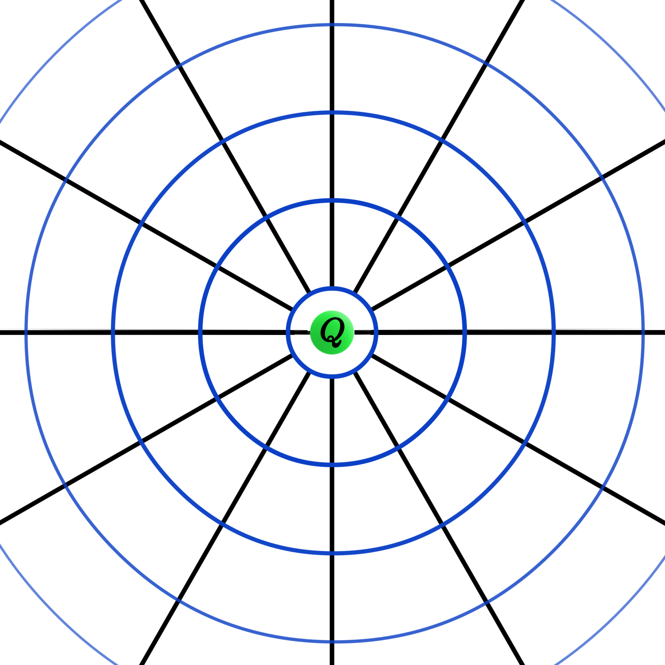
Whereas the electric field lines emanate radially away from the charge, the magnetic field lines circle around it. And together, the two fields look something like a wheel and its spokes, when viewed from head-on.

In fact, there's a simple relationship between the two fields in this case: the magnetic field, $\vec B,$ is given by the cross product between the particle's velocity vector and the electric field, up to a factor of the speed of light: $$ \vec B = \frac{1}{c^2} \vec v \times \vec E. $$

I'll continue to mainly discuss the electric field here, so that we can focus on one thing at a time. But know that electricity is really just one half of the larger subject of electromagnetism.

The Field of an Accelerating Charge

At last, we come to the most challenging—but also the most fascinating—variety of electric field: the field produced by an accelerating charge.

We started off with the simple, radial field of a charge sitting at rest. And from there, we generalized to the electric field of a charge moving at constant velocity. The field still pointed radially away from the particle, albeit with a non-uniform angular distribution.

But now, we'll finally allow our charge to accelerate. And in doing so, we'll discover that the field must carry out waves of information that communicate the state of the charge to the rest of the universe.

To focus on perhaps the simplest example, suppose our charge is initially sitting at rest at the origin, until somebody comes along and gives it a sharp kick at time $t = 0$, rapidly accelerating it to a relativistic speed $v$.

Then what does the electric field of the charge look like both before and after that abrupt burst of acceleration?

Beforehand, the charge has just been sitting at rest at the origin, and so it sources the usual Coulomb field that we started with from the very beginning. A short time after the kick, though, we'll find the particle traveling to the right with its new speed $v$.

And given what we just discussed, you might guess that the charge is then going to drag along that same Coulomb field—maybe squished a bit along the direction of motion, depending on how close $v$ is to the speed of light.

But that's wrong. That was the field for a charge that's been moving at constant velocity forever. Not one that's been suddenly accelerated up to speed $v$.

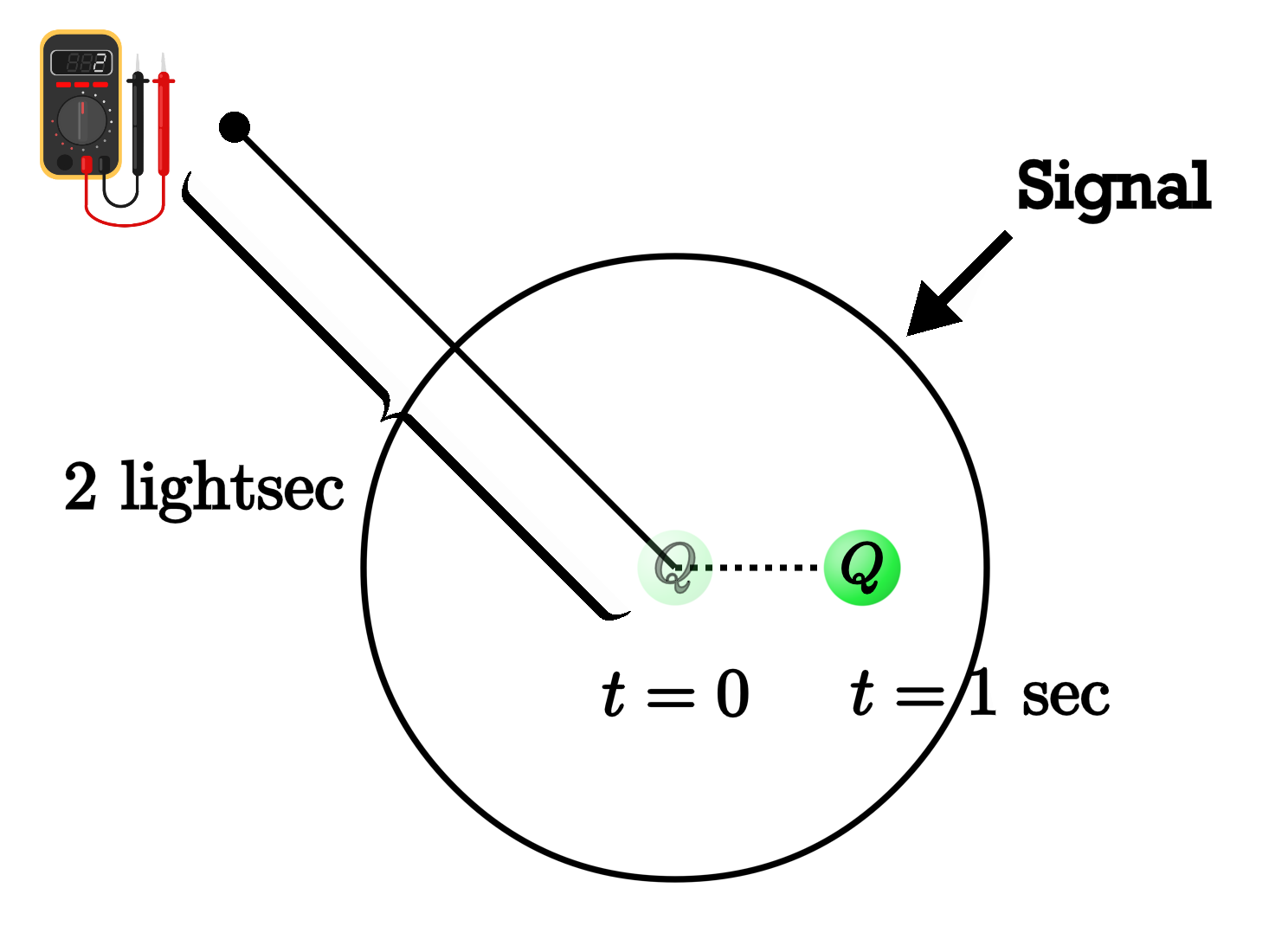
And we can see that it's wrong for a very simple reason. Suppose we go to draw what the field looks like at $t = 1$ second after the initial kick. Picture yourself standing with your electric field meter at a point that's a fair distance away from the origin—let's say it's 2 light-seconds away. Then at this moment, the news that the particle has suddenly started moving hasn't even reached you yet.

It can't have, because a light signal emitted from the origin at $t = 0$ has only managed to travel half that distance in the intervening second. As far as you know from so far away, the charge is still sitting at rest at the origin, and the electric field that you measure can't have changed at all yet.

Instead, from the moment of the kick at $t=0$, the news that the particle has accelerated radiates away from the origin in a spherical shell that expands outward at the speed of light—that is, with radius $r = ct$.

At any point outside the shell, nothing's changed yet compared to the state of the field before the kick. The field lines still point radially away from where the charge was at the origin for all the long time before the clock struck $t = 0$.

Inside the shell, on the other hand, the news that the particle is now moving has arrived. And in this region, the field does look very much like what we just discussed for the field lines of a charge moving with constant velocity $v,$ pointing radially away from the current position of the particle.

All that we can deduce about the field of this accelerating charge solely on the basis of causality—that no signal can travel faster than the speed of light.

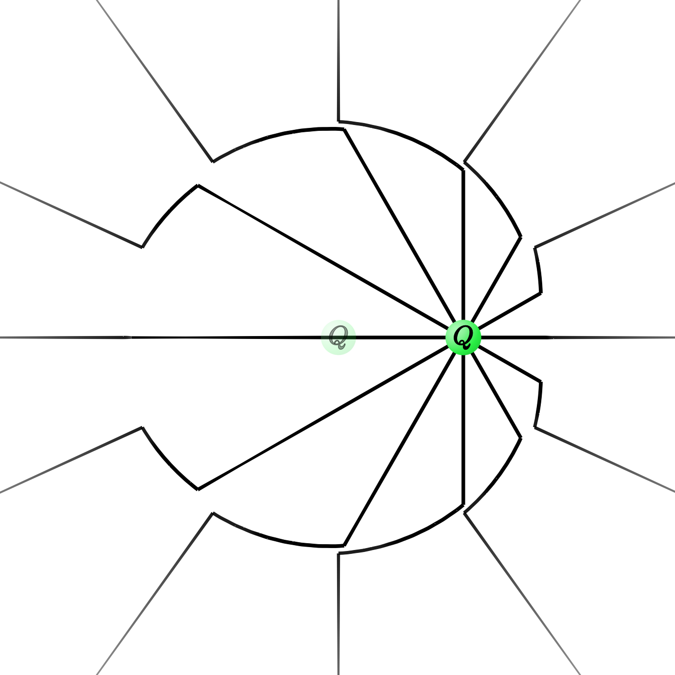
What's even more interesting, though, is how the field behaves in between those two regions—in the vicinity of the expanding shell. The outer field lines of the charge that was at rest at the origin must smoothly connect to the inner field lines of the charge in motion. And there's really only one way that they can: in zig-zagging arcs that run almost tangent to the shell.

Combined with the magnetic component, those expanding zig-zags are the electromagnetic wave radiated out from the origin that communicates the news of the particle's acceleration. In other words, an accelerating charge must produce an electromagnetic wave—a ripple in the electric and magnetic fields—that expands outward at the speed of light.

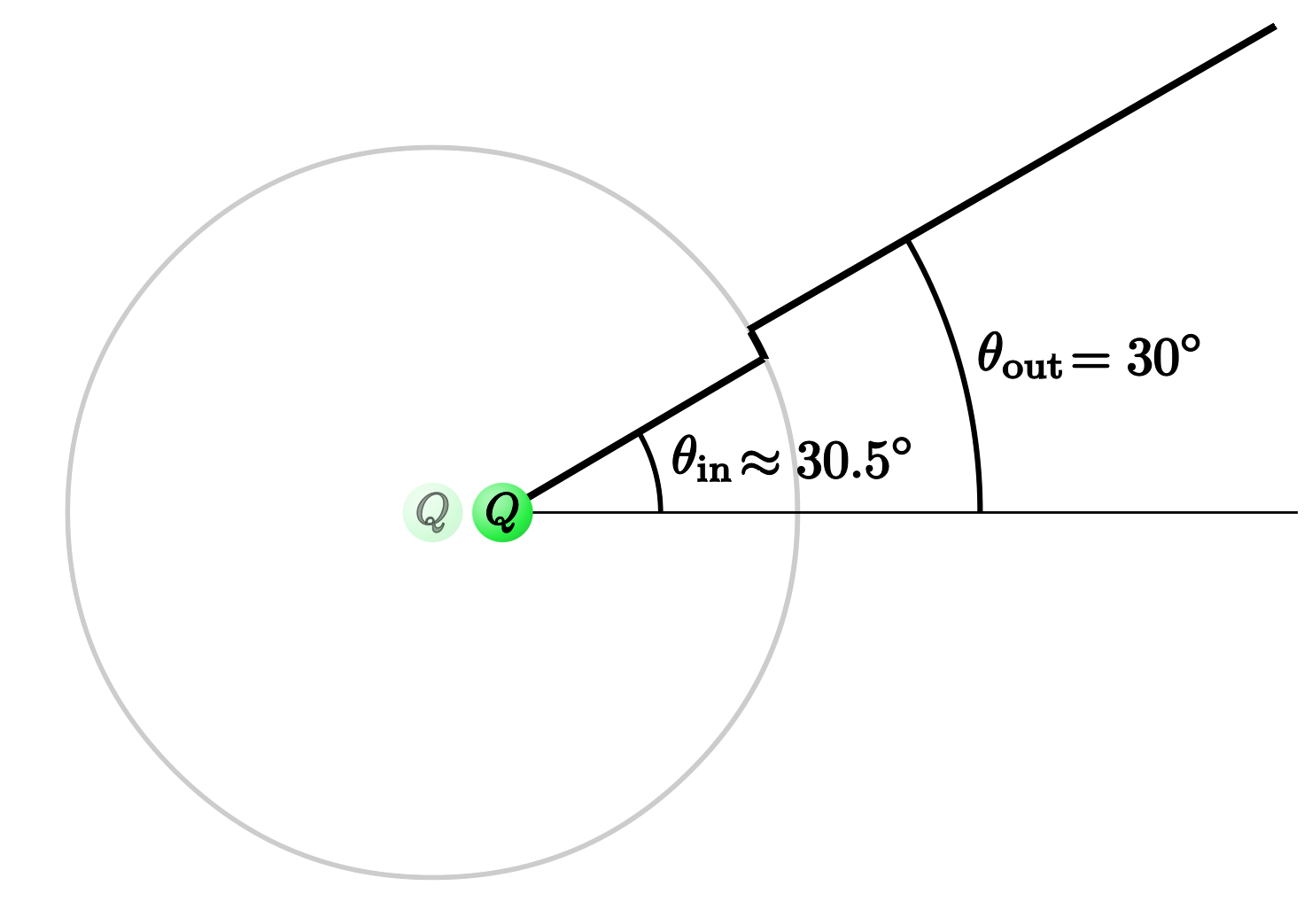
To understand why the zig-zagging lines take the shape that they do, consider just one line that emerges from the charge at some angle $\theta_\mathrm{in}$ inside the shell. It extends radially away from the charge until it hits that boundary, and then emerges at some new angle $\theta_\mathrm{out}$ outside the shell, extending radially away from the origin.

And again, in between, there's only one way the field line can go: tangentially along the arc of the circle.

There's one thing causality alone doesn't tell us, though. Given the initial angle of the field line inside the shell, what angle does it wind up at when it emerges on the outside? To answer that question, we turn once more to Gauss's law, with a clever choice for the surface $\mathrm S.$

Picking a starting point a distance $R_\mathrm{in}$ from the current location of the charge inside the shell, imagine following the field line until we emerge at some point on the outside at a distance $R_\mathrm{out}$ from the origin. By construction then, the electric field points parallel to that path everywhere along it.

Meanwhile, at the two ends of the segment, we can draw circular arcs that connect back down to the horizontal axis—the inner arc being centered at the current location of the charge, while the outer arc is centered at the original location at the origin. Along those arcs, the electric field is then perpendicular to the path.

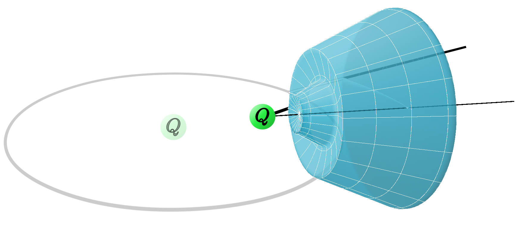
By revolving that curve around the axis of motion, we obtain a closed surface, $\mathrm S$. But crucially, it's a surface that contains no charge anywhere inside of it. And Gauss's law therefore says that the total flux of the electric field passing through the surface must vanish.

The way we've constructed it, though, the only contributions to that flux come from the inner and outer caps of the surface, where the field is perpendicular to it. And therefore the flux passing into the inner cap must cancel against the flux going out through the outer cap, so that the total adds up to zero.

$$ \Phi_\mathrm{in}=- \Phi_\mathrm{out}. $$

By evaluating those two fluxes, we'll then be able to determine the relationship between $\theta_\mathrm{in}$ and $\theta_\mathrm{out}.$

The flux through the outer cap is due to the Coulomb field that the charge produced when it was at rest at the origin:

$$ \Phi_\mathrm{out} = \frac{Q}{4\pi\epsilon_0} \int \frac{\hat r}{R_\mathrm{out}{}^2} \cdot \hat r\, R_\mathrm{out}{}^2 \sin(\theta)\, \mathrm d \theta \, \mathrm d\phi. $$

Here, we're integrating over a patch of a sphere of radius $R_\mathrm{out}$ surrounding the origin, where $\theta$ runs from $0$ to $\theta_\mathrm{out}$ and $\phi$ runs from $0$ to $2\pi$. As before, there are no factors of $\phi$ in the integrand, and so that integral just contributes a factor of $2\pi$:

$$ \Phi_\mathrm{out} = \frac{Q}{2\epsilon_0} \int_0^{\theta_\mathrm{out}}\mathrm d \theta \, \sin \theta . $$

We therefore obtain

$$ \Phi_\mathrm{out} = \frac{Q}{2\epsilon_0} (1 - \cos \theta_\mathrm{out}) $$

for the flux passing through the outer cap of the surface. Note that in the limit $\theta_\mathrm{out} = \pi,$ the outer cap becomes a complete sphere of radius $R_\mathrm{out}$ enclosing the particle, and we obtain $\Phi_\mathrm{out} = Q/\epsilon_0$ in accordance with Gauss's law.

The flux passing in through the inner cap, on the other hand, is due to the field of the moving charge:

$$ \Phi_\mathrm{in} = -\frac{Q}{4\pi\epsilon_0} \int \frac{1 - v^2/c^2}{(1 - \sin^2(\theta)\, v^2/c^2)^{3/2}} \frac{\hat R}{R_\mathrm{in}{}^2} \cdot \hat R~ R_\mathrm{in}{}^2 \sin(\theta)\, \mathrm d \theta \mathrm \,\mathrm d \phi, $$

where now we're integrating over the patch of a sphere of radius $R_\mathrm{in}$ surrounding the current location of the charge. Note the overall minus sign, which appears because this flux is passing into the surface rather than flowing out from it.

Simplifying, we get

$$ \Phi_\mathrm{in} = -\frac{Q}{2\epsilon_0} (1-v^2/c^2) \underbrace{\int_0^{\theta_\mathrm{in}} \mathrm d \theta\, \frac{\sin(\theta)}{(1 - \sin^2(\theta)\, v^2/c^2)^{3/2}}}_{\frac{1}{1-v^2/c^2} \left( 1 - \frac{\cos(\theta_\mathrm{in})}{\sqrt{1 - \sin^2(\theta_\mathrm{in})\, v^2/c^2}} \right)} . $$

The flux passing into the inner cap is then

$$ \Phi_\mathrm{in} = -\frac{Q}{2\epsilon_0} \left( 1 - \frac{\cos(\theta_\mathrm{in})}{\sqrt{1 - \sin^2(\theta_\mathrm{in})\, v^2/c^2}} \right). $$

Again, since there's no charge contained within the surface, Gauss's law says that these two fluxes must cancel each other out:

$$ \frac{Q}{2\epsilon_0} \left( 1 - \frac{\cos(\theta_\mathrm{in})}{\sqrt{1 - \sin^2(\theta_\mathrm{in})\, v^2/c^2}} \right) = \frac{Q}{2\epsilon_0} (1 - \cos \theta_\mathrm{out}). $$

In this way, Gauss's law has told us the relationship between the inner and outer angles of the field line, and the speed $v$ of the particle:

$$ \frac{\cos(\theta_\mathrm{in})}{\sqrt{1 - \sin^2(\theta_\mathrm{in})\, v^2/c^2}} = \cos (\theta_\mathrm{out}). $$

This relation can be simplified by squaring and inverting both sides:

$$ \frac{1 - \sin^2(\theta_\mathrm{in})\, v^2/c^2}{\cos^2(\theta_\mathrm{in})} = \frac{1}{ \cos^2 (\theta_\mathrm{out})}. $$

Replacing $v^2/c^2 = 1 - 1/\gamma^2$ and simplifying, we obtain

$$ 1 + \frac{1}{\gamma^2} \tan^2(\theta_\mathrm{in}) = \frac{1}{ \cos^2 (\theta_\mathrm{out})}. $$

Applying the identity $$ \begin{aligned} &\tan^2(\theta_\mathrm{out}) = \frac{1}{\cos^2(\theta_\mathrm{out})} - 1, \end{aligned} $$

we learn that

$$ \tan^2(\theta_\mathrm{out}) = \frac{1}{\gamma^2} \tan^2(\theta_\mathrm{in}). $$

We've therefore established the following simple relationship between the inner and outer angles of the field lines:

$$ \tan(\theta_\mathrm{in}) = \gamma \tan(\theta_\mathrm{out}). $$

The outer angles are of course uniformly distributed, since they correspond to the usual Coulomb field lines. If the particle isn't moving too fast compared to the speed of light, then $\gamma$ is close to 1, and the inner angles are almost identical to the outer angles:

$$ \theta_\mathrm{in} \overset{v/c \ll 1}{\longrightarrow} \theta_\mathrm{out}. $$

For example, when $v = 0.2c$ as pictured below, a field line that makes a $30^\circ$ angle outside the shell connects to one that's likewise at about $30^\circ$ inside the shell.

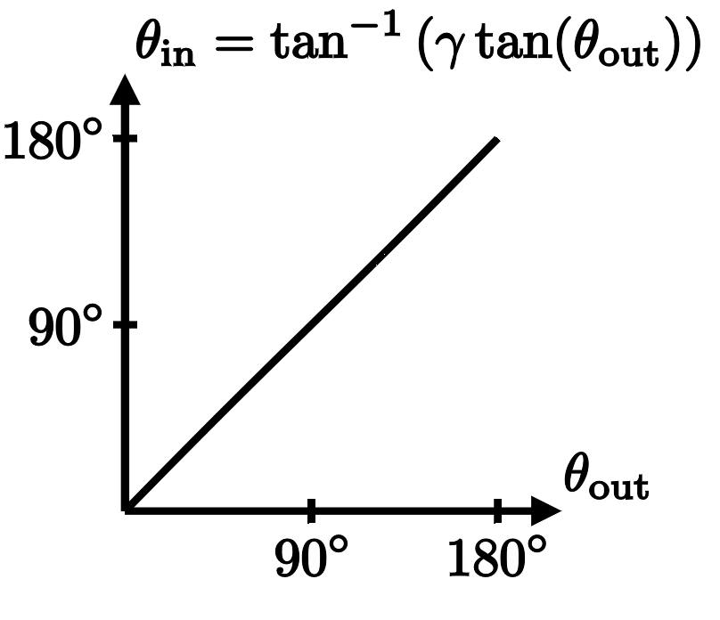
In this limit where $v/c$ is small, if we draw a plot of the inner angle versus the outer angle, it's very nearly a straight line of slope one, $\theta_\mathrm{in} \approx \theta_\mathrm{out}$:

However, as the particle approaches the speed of light, the plot of $\theta_\mathrm{in} = \tan^{-1}(\gamma \tan(\theta_\mathrm{out}))$ begins to flatten out with a horizontal plateau at $90^\circ$. Meaning that all the outer field lines in that ever-widening range emerged from the particle at very nearly a right angle:

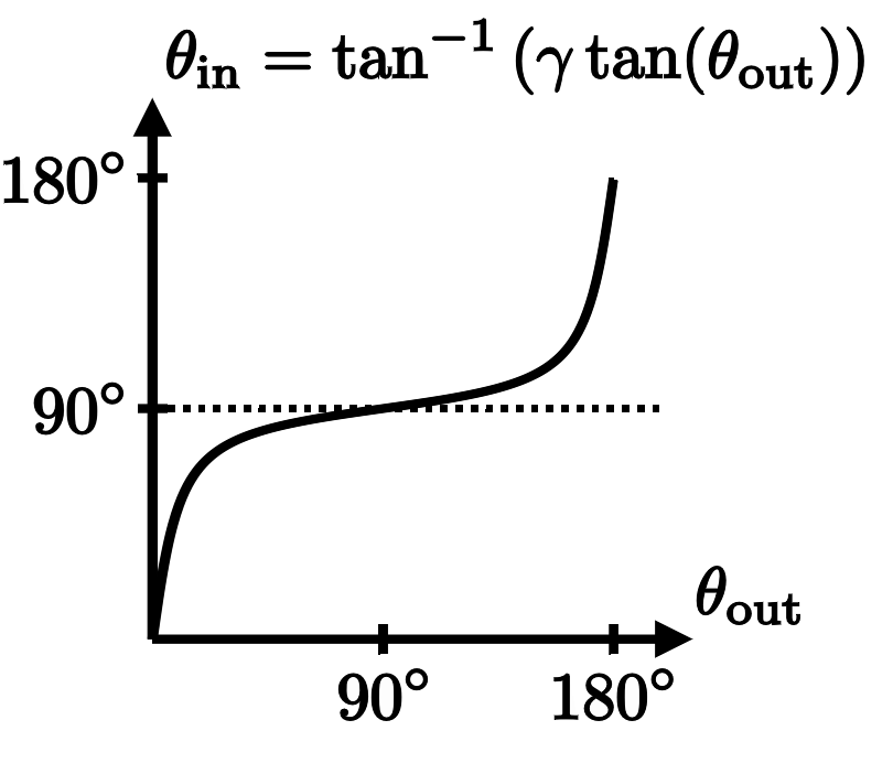
And that's exactly what we should expect! Because, as we just learned, the electric field of a particle traveling at nearly light speed is squished along its direction of motion, with most of its field lines concentrated at right angles to the velocity.

We've come a very long way from the simple Coulomb field of an electric charge sitting at rest, to understand not just the field of a moving charge, but of one that's accelerating as well.

And I hope these arguments have convinced you that it had to be this way. That since information can't instantaneously travel from one side of the universe to the other, any accelerating charge must radiate waves in the electromagnetic field that ripple outward as fast as they can—but no faster.